A-NICE-MC: Adversarial Training for MCMC
TLDR: A brief introduction to our NIPS 2017 paper, A-NICE-MC: Adversarial Training for MCMC, where we introduce a method to train flexible MCMC proposals (parameterized by neural networks) that are provably correct and much more efficient than typical hand-crafted ones.
Bayesian Inference is a key paradigm in AI and machine learning. The goal is to estimate a posterior distribution over models \(p(\theta \vert x)\), given a prior \(p(\theta)\) and a data likelihood \(p(x \vert \theta)\), through Bayes’ rule:
\[\underbrace{p(\theta \vert x)}_{posterior} \propto \underbrace{p(\theta)}_{prior} \underbrace{p(x \vert \theta)}_{likelihood}\]Unfortunately, the posterior is often intractable to compute, hence approximations are used in practice. There are two major paradigms for approximate inference: Variational Inference and Markov Chain Monte Carlo (MCMC) methods. In variational inference, the posterior is approximated with a simpler distribution: the problem is reduced to an optimization one, where the objective is to minimize some notion of distance between the posterior and a family of approximating distributions. In MCMC, the posterior is approximated with a set of particles, obtained by simulating a Markov chain. Variational inference methods are more efficient computationally but are limited by the expressiveness of the approximating family. MCMC methods, on the other hand, are generally slower but have the appealing property that they are asymptotically exact in the limit of infinite samples.
In recent years, there has been enormous progress in variational inference methods. One of the reasons is that because inference is reduced to an optimization problem, it can easily benefit from the use of expressive deep neural networks, automatic differentiation, and stochastic gradient descent. MCMC methods, on the other hand, have not benefited as much from these advances. MCMC methods typically use Markov Chains that are hand-designed, and generally do not involve a large number of tunable parameters; even if they do, MCMC performance metrics are difficult to quantify and thus optimize directly.
In this blog post we describe a new approach to automatically obtain more efficient MCMC proposals. Instead of using domain-agnostic and hand-crafted Markov Chains, we consider a flexible class of chains that are parametrized with neural networks and can be tuned to specific application domains. The network is trained through a novel adversarial training method which allows the discovery of efficient Markov Chains for posterior sampling. As we will demonstrate in the experiments, the learned chains allow us to generate posterior samples far more efficiently than state-of-the-art hand-crafted proposals such as Hamiltonian Monte Carlo (HMC).
Background: Markov Chain Monte Carlo
Consider the following problem:
Given a distribution with some (un-normalized) analytical form \(p(x) \propto \exp(-U(x))\), how can we sample from it efficiently?
Even with the analytical expression, direct sampling is difficult. The idea of MCMC methods is to instead set up a Markov Chain such that if we were to simulate this chain for a sufficiently large number of steps, the chain would ultimately converge (in distribution) to \(p(x)\) (its stationary distribution).
The Metropolis-Hastings (MH) algorithm, one of the most important algorithms of all time, provides a recipe to construct such a Markov chain given the un-normalized density. In MH, the user specifies an arbitrary proposal1 \(g(x' \vert x)\) that proposes a new sample \(x'\) given the previous sample \(x\). The algorithm then uses the following distribution to accept or reject the proposed sample:
\[A(x' \vert x) = \min (1, \frac{p(x')g(x\vert x')}{p(x) g(x' \vert x)}) = \min (1, \frac{g(x\vert x')}{g(x' \vert x)} \exp(U(x) - U(x')))\]The transition kernel of the resulting Markov Chain, i.e., the probability of transitioning from a state \(x\) to a new state \(x'\), would then have the form \(q(x' \vert x) = g(x' \vert x) A(x' \vert x)\). One can show that \(q(x' \vert x)\) always satisfies detailed balance, namely:
\[q(x' \vert x) p(x) = q(x \vert x') p(x')\]and that the stationary distribution of the chain \(q(x' \vert x)\) is always \(p(x)\). In other words, regardless of how the proposal is chosen, asymptotically this Markov Chain will spend the right amount of time in each state \(x\), i.e., proportional to \(p(x)\).
Metropolis-Hastings is the crux of most Markov Chain Monte Carlo (MCMC) methods (Brooks et al. 2011), and is widely used in Bayesian statistics, computational physics, computational biology and graphics. However, Metropolis-Hastings does not tell us anything about the convergence rate to the stationary distribution, which in fact depends heavily on the proposal used for sampling. Therefore, the selection of a good proposal is a crucial problem in MCMC. Unfortunately, selection of a good proposal is particularly hard, because convergence to the stationary is difficult to detect, and it is therefore hard to tell which proposals are “good”. Popular metrics to evaluate MCMC performance include Effective Sample Size (ESS) and Gelman-Rubin diagnostic 2.
This leads to the following problem:
Is it possible to automatically choose a reasonably “good” proposal for a specific distribution \(p(x)\)?
In this post, we discuss an approach to achieve this. Our learned proposals are significantly more effective than hand-crafted proposals such as HMC, as shown in the following figure where we can quickly recover the target distribution \(p(x)\):
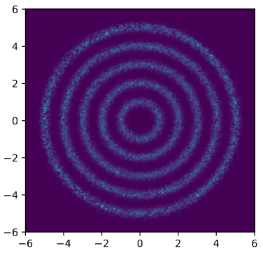
(Left) Target distribution, which consists of multiple rings. (Middle) Sampling with HMC. (Right) Sampling with A-NICE-MC. A-NICE-MC performs much better than HMC.
Similar to black-box variational inference (Ranganath, Gerrish, and Blei 2014) which bridges the gap between variational inference and deep learning, we intend to bridge the gap between MCMC and deep learning, enabling the use of flexible proposals parameterized by neural networks.
Adversarial Training of Markov Chains
Suppose we have a flexible family of proposals parameterized by \(\theta\), e.g., with a neural network. For example, \(g(x' \vert x)\) could be a Gaussian with mean and standard deviation given by a feed-forward neural network taking \(x\) as input.
Let \(\pi_0\) to be an initial state distribution, \(\pi_t\) to be the state distribution at time step \(t\) and \(\pi_\theta = \lim_{t \to \infty} \pi_t\) to be the stationary distribution (assuming it exists). Using MH, we can guarantee that the stationary distribution is correct for any choice of \(\theta\). However, to achieve fast convergence we would also like \(\pi_t\) to be close to the target \(p\), for some small value of \(t\).
The challenge is that evaluating probabilities with respect to \(\pi_t\) – computing the probability of a state at time \(t\) – requires integration of all the possible paths of length \(t\) leading to that state. This rules out any kind of likelihood-based method. However, sampling from \(\pi_t\) is relatively straightforward.
We therefore propose to train the model with likelihood-free methods. The intuition is that if the chain has indeed converged to \(p\) after \(t\) steps, then the distribution at time \(t+1\) should also be \(p\). Therefore, states visited after \(t\) steps should be indistiguishable from states visited after \(t+1\) steps.
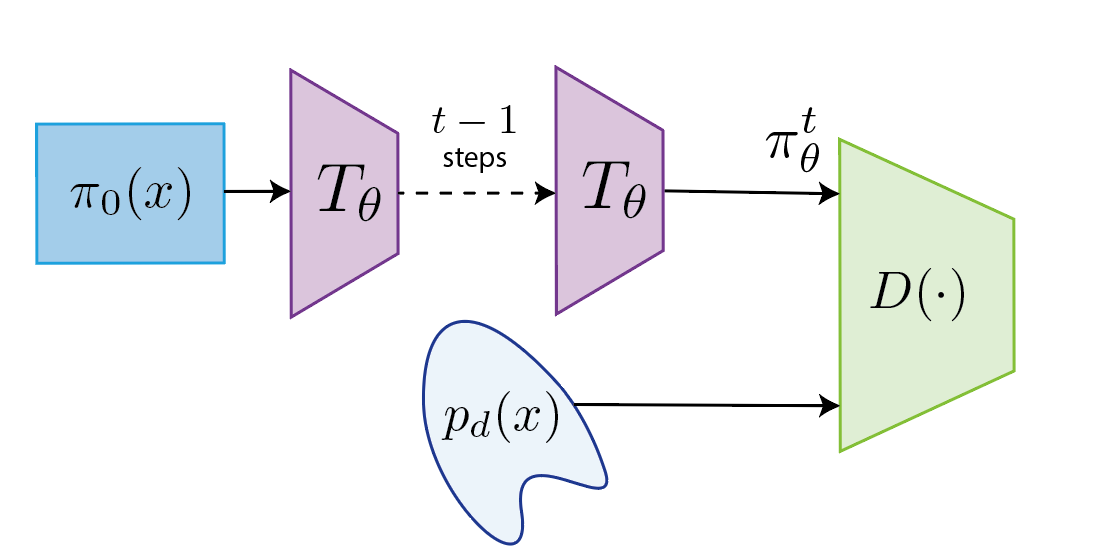
In particular, we use adversarial training (Goodfellow et al. 2014), which involves a two player game between a discriminator \(D\) and a generator \(G\). The discriminator aims to discriminate samples from the generator and samples from a target distribution \(p_d\) (that can be easily sampled from), whereas the generator aims to fool the discriminator, leading to the following minimax objective3:
\[\min_G \max_D \mathbb{E}_{x \sim p_d}[D(x)] - \mathbb{E}_{x \sim G}[D(x)]\]In our case, the generator \(G\) can be defined from the transition operator \(T_\theta\) applied \(t\) times 4. If we could choose \(p_d=p\), we would enforce convergence of the resulting Markov Chain to the desired stationary distribution \(p\) in \(t\) steps. Unfortunately, optimizing the above objective requires samples from \(p_d=p\), which we don’t have.
Bootstrap
Ideally, we would like to optimize the above objective using a set of samples from \(p(x)\) – this is how these techniques are typically used; however, in our case we are provided with the analytical form of \(p\) instead of samples, and obtaining samples is the whole purpose of MCMC!
To overcome this challenge and obtain samples from \(p(x)\), we consider a bootstrap process:
- Initially, we obtain samples from a “bad” chain, which still converges to \(p(x)\) if sampled indefinitely. However, we only run the chain for \(T\) steps.
- We train our generator (by optimizing the transition operator) with these samples and \(t \ll T\). Effectively, we attempt to accomplish in \(t\) steps what the “bad” chain did in \(T \gg t\) steps, yielding a “better” chain.
- We then repeat the process using samples obtained with this new, “better” chain.
In other words, this procedure allow us to obtain better samples and better proposals iteratively.
Metropolis-Hastings with A NICE Proposal
The only remaining step is to define a suitable class of proposals, which have the following requirements:
- We need to be able to sample from it efficiently.
- We need to be able to evaluate likelihoods according to the proposal to perform Metropolis-Hastings.
- The proposal should be differentiable objective with respect to \(\theta\) to enable gradient-based optimization.
A seemingly natural choice is to set the proposal \(g(x' \vert x)\) to be a Gaussian with mean and standard deviation given by a feed-forward neural network taking \(x\) as input. With this proposal, we can obtain samples from the corresponding MCMC chain and optimize the adversarial loss with score-function gradient estimators (such as REINFORCE). However, we found this method fails completely due to extremely low acceptance rates at the beginning of the training process.
To see this, let’s consider the \(g(x \vert x') / g(x' \vert x)\) term in the expression for the acceptance probability. Then to have \(g(x \vert x')\) match \(g(x' \vert x)\) intuitively means that running the proposal twice should return to the original state, which is hard to satisfy in practice.
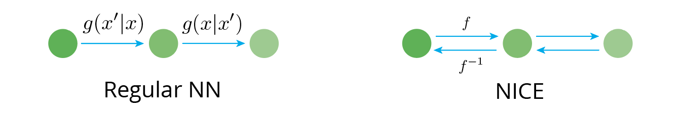
Therefore, the above approach would fail since \(g(x \vert x') / g(x' \vert x)\) tends to be too small, leading to low acceptance rates. As an alternative, we could use NICE where the value of \(g\) does not affect the acceptance rate.
We utilize a special type of neural network architecture called NICE (Dinh, Krueger, and Bengio 2014). The NICE network is invertible and volume-preserving (the determinant of the Jacobian is 1). This property is particularly useful for constructing parametrized neural network proposals that belong to the “implicit” category.
Let \(f(x, v)\) be the NICE network we wish to incoporate in our proposal, where \(v\) is an auxiliary variable we sample independently from \(x\) at every step. We consider the following proposal, which we term a “NICE proposal”:
- With probability 1/2, let \(x', v' = f(x, v)\)
- With probability 1/2, let \(x', v' = f^{-1}(x, v)\)
We can easily prove that \(g(x', v'\vert x, v) = g(x, v\vert x', v')\). Therefore, we only need to consider \(U(x, v) = U(x) + U(v)\) during the Metropolis-Hastings step:
\[\begin{align} A(x', v' \vert x, v) = \min (1, \exp(U(x, v) - U(x', v'))) \end{align}\]which holds for any specific parametrization of the NICE network.
How do NICE proposals connect to learning MCMC proposals? Interestingly, we can train the NICE proposal with the forward mapping \(f\) only, for the target \(p(x, v) = p_d(x) p(v)\), so the training procedure reduces to the fully-differentiable one. The following figure intuitively demonstrates why we could do this.
Since the NICE network is invertible, if the forward operation \(f\) moves a point from \(p(x, v)\) to another point from \(p(x, v)\), then the backward operation will do the same. Meanwhile, the forward operation will encourage the points to move toward \(p(x, v)\) and \(A\) tends to reject backward operations that move away from \(p(x, v)\), thereby removing random-walk behavior from happening during burn-in.
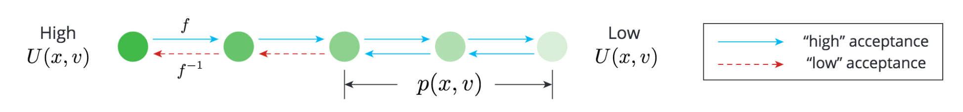
We can obtain a good MCMC proposal by training the forward process only.
This provides an automated process of training a domain-specific MCMC kernel that converges to the stationary quickly 5. We name the resulting process A-NICE-MC (Adversarial NICE Monte Carlo).
Empirical Results
In the first case, we consider simple 2-D distributions that are easy to visualize. If there are multiple modes that are far from each other, HMC can fail to move between the modes efficiently, and in some cases it does not converge to the target distribution even with multiple chains. A-NICE-MC, on the other hand, is able to move across these modes easily with neural network proposals.
Sampling from distributions with multiple modes with A-NICE-MC (in gif).
In the second case, we consider posterior inference for Bayesian Logistic regression, which has a single mode and for which HMC is a strong baseline. While HMC outperforms A-NICE-MC in terms of ESS, the fact that it computes gradient information makes it slower to compute, and that A-NICE-MC actually outperforms HMC in terms of ESS per second since it does not compute \(\nabla U(x)\). Moreover, we tune the parameters for HMC in different dataset while using the same set of parameters for A-NICE-MC.
| ESS | A-NICE-MC | HMC |
|---|---|---|
| german | 926.49 | 2178.00 |
| heart | 1251.16 | 5000.00 |
| australian | 1015.75 | 1345.82 |
| ESS / s | A-NICE-MC | HMC |
|---|---|---|
| german | 1289.03 | 216.17 |
| heart | 3204.00 | 1005.03 |
| australian | 1857.37 | 289.11 |
ESS and ESS per second for Bayesian logistic regression tasks.
Discussion
In this blog post, we introduced the first likelihood-free method for training the transition operator of a Markov Chain, and ways to bridge the gap between MCMC and deep learning.
Here is a related follow-up work by Google Brain: (Levy, Hoffman, and Sohl-Dickstein 2017) which uses expected square jump distance (Pasarica and Gelman 2010) to optimize for lag-1 autocorrelation.
The code for reproducing our experiments is available at https://github.com/ermongroup/a-nice-mc.
Footnotes
-
Making some mild assumptions, e.g. the proposal is ergodic and irreducible. ↩
-
We mostly consider ESS and ESS per second in the paper. However, we also evaluated the Gelman’s R hat diagnostic (Brooks and Gelman 1998), which evaluates performance across multiple sampled chains – we still outperform HMC in this metric. ↩
-
We use the Wasserstein GAN objective here (Arjovsky, Chintala, and Bottou 2017). ↩
-
The objective used in our paper is slightly different – we consider two necessary conditions and used that for the objective, which is computationally more efficient. ↩
-
To train for higher ESS we need to use a pairwise discriminator, which takes a pair of samples as input; please refer to our paper and code for more details. ↩
References
- Brooks, Steve, Andrew Gelman, Galin Jones, and Xiao-Li Meng. 2011. Handbook of Markov Chain Monte Carlo. CRC press.
- Ranganath, Rajesh, Sean Gerrish, and David Blei. 2014. “Black Box Variational Inference.” In Artificial Intelligence and Statistics, 814–22.
- Goodfellow, Ian, Jean Pouget-Abadie, Mehdi Mirza, Bing Xu, David Warde-Farley, Sherjil Ozair, Aaron Courville, and Yoshua Bengio. 2014. “Generative Adversarial Nets.” In Advances in Neural Information Processing Systems, 2672–80.
- Bengio, Yoshua, Eric Laufer, Guillaume Alain, and Jason Yosinski. 2014. “Deep Generative Stochastic Networks Trainable by Backprop.” In International Conference on Machine Learning, 226–34.
- Dinh, Laurent, David Krueger, and Yoshua Bengio. 2014. “NICE: Non-Linear Independent Components Estimation.” ArXiv Preprint ArXiv:1410.8516.
- Levy, Daniel, Matthew D Hoffman, and Jascha Sohl-Dickstein. 2017. “Generalizing Hamiltonian Monte Carlo with Neural Networks.” ArXiv Preprint ArXiv:1711.09268.
- Pasarica, Cristian, and Andrew Gelman. 2010. “Adaptively Scaling the Metropolis Algorithm Using Expected Squared Jumped Distance.” Statistica Sinica, 343–64.
- Brooks, Stephen P, and Andrew Gelman. 1998. “General Methods for Monitoring Convergence of Iterative Simulations.” Journal of Computational and Graphical Statistics 7 (4): 434–55.
- Arjovsky, Martin, Soumith Chintala, and Léon Bottou. 2017. “Wasserstein GAN.” In International Conference on Machine Learning.