Bias and Generalization in Deep Generative Models
Generative Models and Generalization
Generative model learning algorithms are designed to learn complex probability distributions from samples. For example, given the set of images in ImageNet [1], we would like to learn a distribution that generates natural images. With recent progress, many types of learning algorithms (such as GANs [2], VAEs and Flow Models [3,4]) can learn distributions whose samples are highly visually appealing images such as the ones below [2].
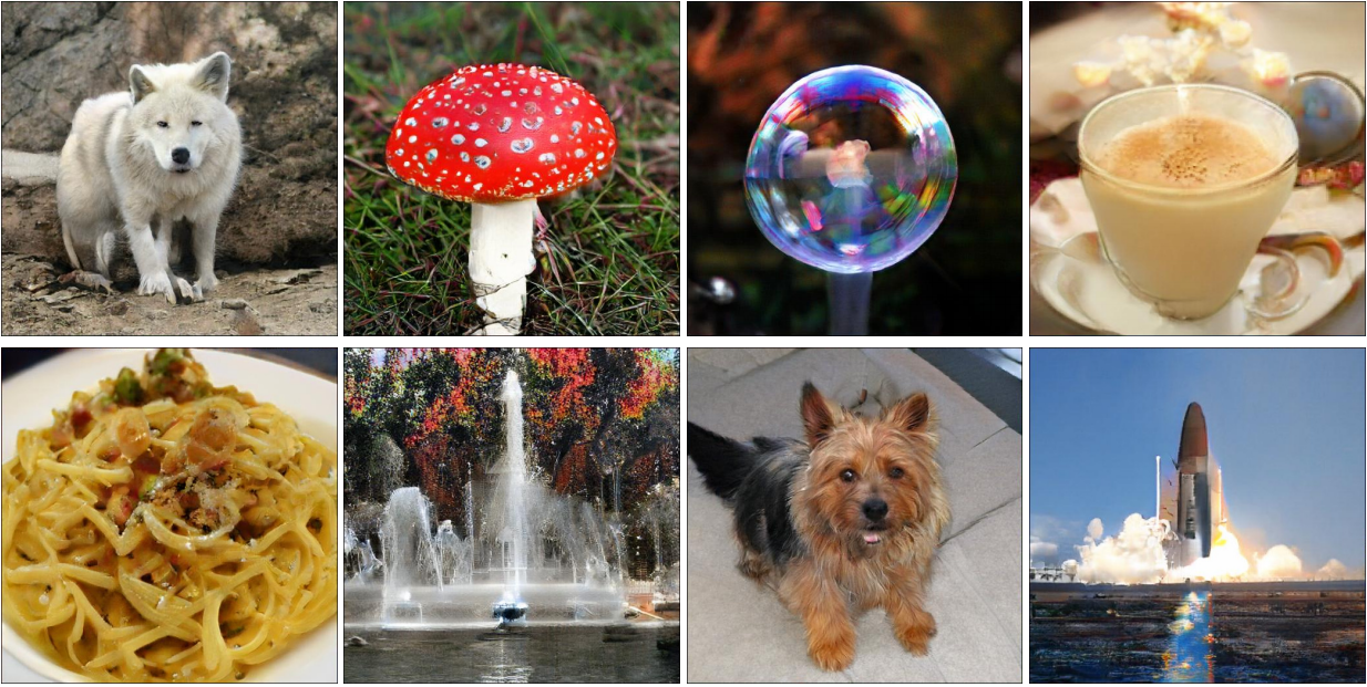
However, the mechanism underlying this amazing performance is poorly understood. But one thing is certain: generative model learning algorithms rely heavily on inductive bias — the assumption by which a learning algorithm extrapolates from training data. The set of possible natural images is combinatorially large (easily in the order of \(2^{\mathrm{millions}}\)), while the training set is absurdly small compared to it. Extrapolating from such a tiny training set certainly requires very strong inductive bias.
This problem is not unique to generative models. Inductive bias is also extremely important for classification algorithms. However, there has been a huge literature, both theoretical and empirical, studying the inductive bias of classification algorithms. On the other hand, the inductive bias of generative model learning algorithms hasn’t attracted enough attention.
Our Framework
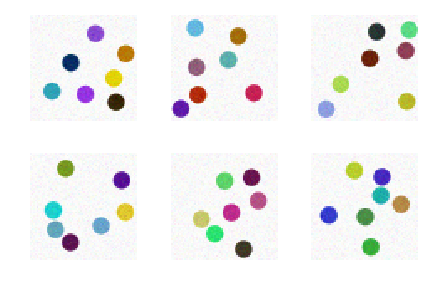
Our paper (ArXiv) (NeurIPS 2018 Spotlight Video) is a framework for the empirical study of the inductive bias of generative model learning algorithms. For example, we can ask questions such as: if every training image contains 2 objects, does the learning algorithm generate images with a different number of objects (e.g. 1 or 3)?

If the training set contains images with red cars, blue cars and red buses, does the learning algorithm generate images with blue buses?

The answer is not obvious, and our framework seeks to answer such questions in a quantitative and reproducible manner.
Empirical Study of Generalization
We start our discussion with one dimensional distributions. We first choose some aspects of the inductive bias. For example, we would like to know the relationship between the variance of the training samples and the variance of the learned distribution. We synthetically design a set of training examples with given variance, and compute the variance of the learned distribution.

By experimenting with several training sets with different variances, we can compare the training set variances and the corresponding learned distribution variances to understand their relationship (for example, we may empirically discover that the learned distribution variance is 10% larger than the training set variance). In addition, this process can be reproduced. We can train different models (e.g., VAEs, GANs, etc.) on these same training sets and compare across different learning algorithms.
To make this methodology effective for high dimensional image data, we need another modification. Several difficulties arise in high dimensions. Understanding the inductive bias is difficult, because there are too many relationships between training samples and learned distributions that we can study. Many properties of the learned distribution are also hard to compute in high dimensions (e.g., entropy, high order moments, etc.).
Therefore, we reduce the high dimensional problem to a low dimensional problem: study the learning algorithm when the image space is projected into a low dimensional feature space. For example, for the object-count feature, we can look at the number of objects in input training images, and the number of objects in the generated samples. In addition, we hope to find aspects of the inductive bias that hold true for different feature spaces.
To provide examples of this methodology, we study three aspects of the inductive biases of common generative model learning algorithms.
Before we present the results, we remark that most results we present here (and in the paper) are qualitatively similar for different learning algorithms (GAN, VAE, Recurrent), architectures (CONV, FC), parameter counts, training set sizes, and hyper-parameters. It is impossible to include everything, but we believe that our selection is sufficiently inclusive, such that these results are most likely valid for typical modern generative models.
Setup 1. Input-Output Relationship of a Single Value of a Single Feature
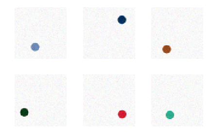
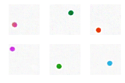
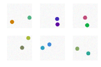
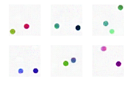
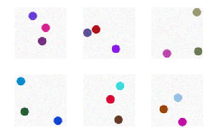
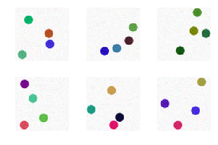
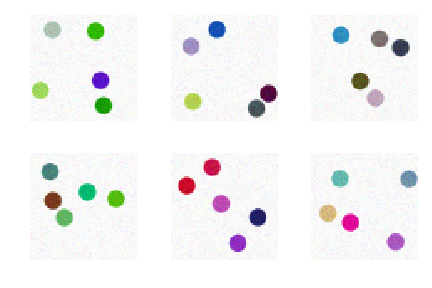
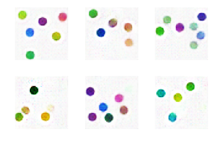
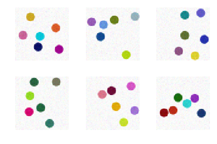
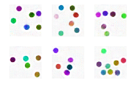
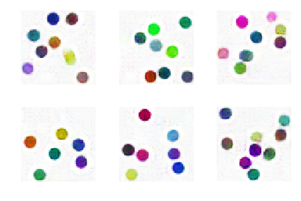
In our first setup, all images in the training set, when projected onto a feature space, take a single value. As an example, we use numerosity (number of objects). For example, if all images in the training set contain 3 objects, will the generated images have a different numerosity? It seems that since the learning algorithm is trained on hundreds of thousands of images — each with 3 objects — it should generate images with 3 objects. Actually this is not true.
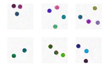
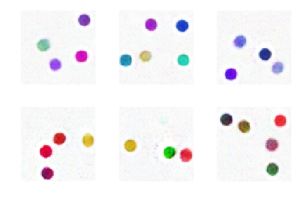
Below we interactively visualize the training images (image with 1-9 dots) and the generated images. Observe that the number of generated dots is often different from the training images.
In the paper we additionally studied other attributes such as color, size, etc, and observed similar trends.
Setup 2. Input-Output Relationship of Multiple Values of a Single Feature
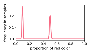
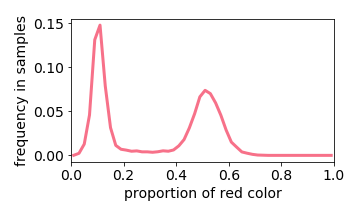
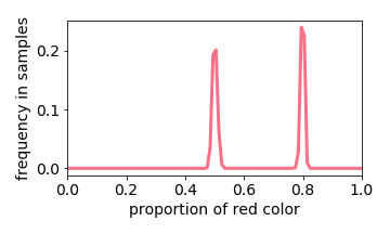
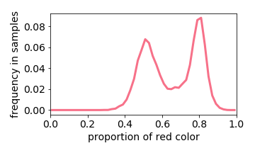
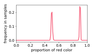
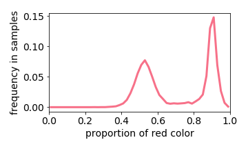
In our second setup, each image in the training set, when projected onto a feature space, takes multiple values. It turns out that the output distribution is very predictable: we take its output distribution for each input value separately (i.e. we studied this in setup 1), and sum them up. In other words, the learning algorithm behaves like a linear filter.
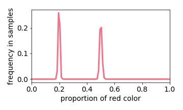
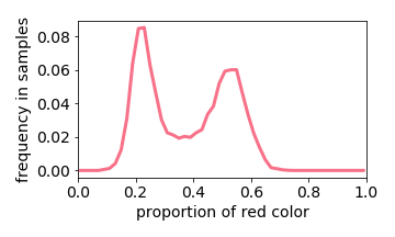
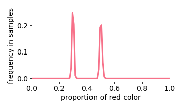
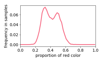
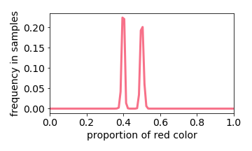
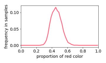
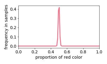
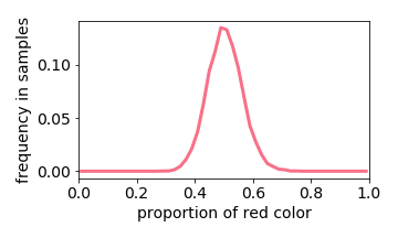
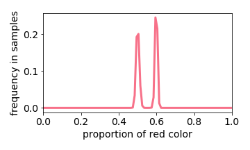
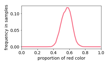
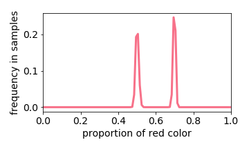
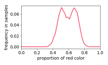
Below we interactive visualize the training samples (e.g. the input image has either 10% or 50% red pixels: it is a distribution with two “spikes”), and the output distribution. Observe how the learning algorithm behaves like a linear filter.
The exception is when two values are close together (e.g. the input image is either 40% or 50% red). The learned distribution will he more concentrated around the mean (e.g. 45% red). This effect is referred to “prototype enhancement” [5] in cognitive psychology.
Setup 3. Combinations of Multiple Features
Finally we study the model’s behavior when there are multiple features. We ask: if we observe some but not all combinations of two features, will the model generate new features. This helps us answer questions such as “will the model generate black swans?”.
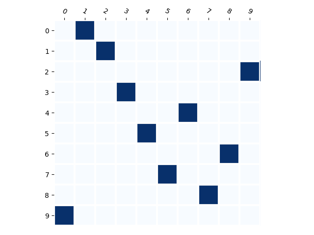
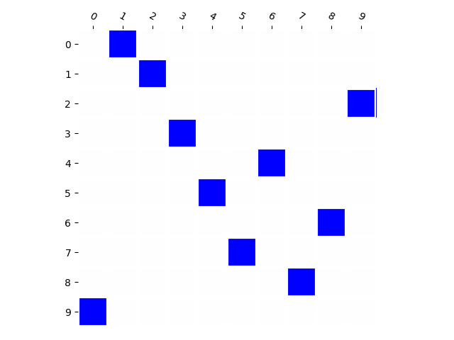
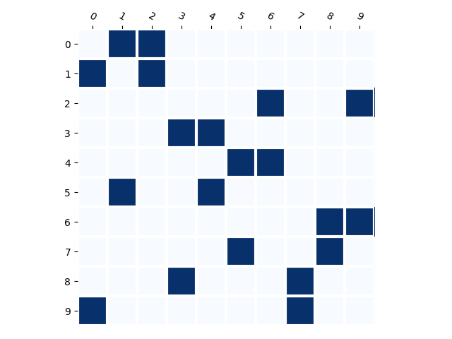
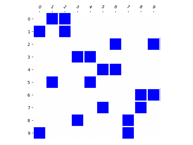
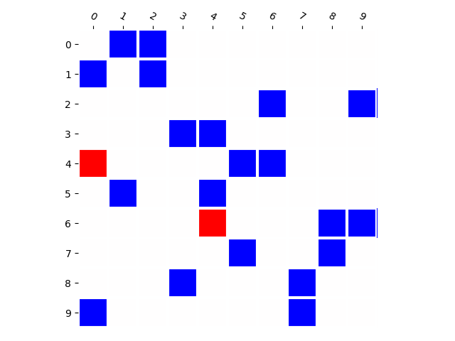
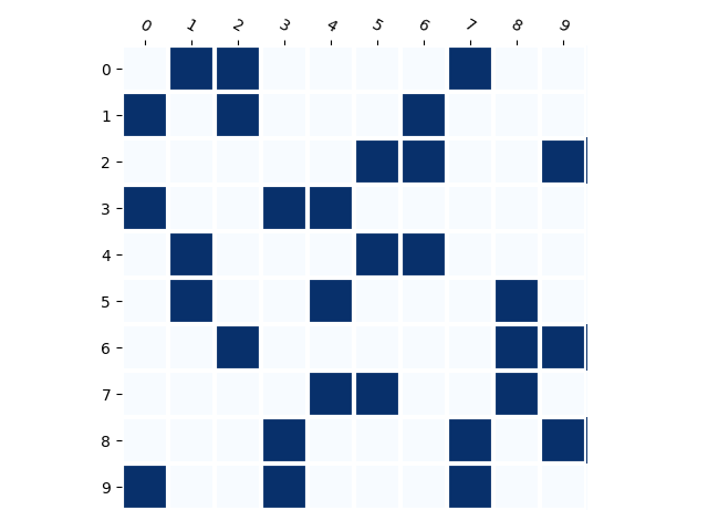
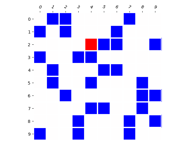
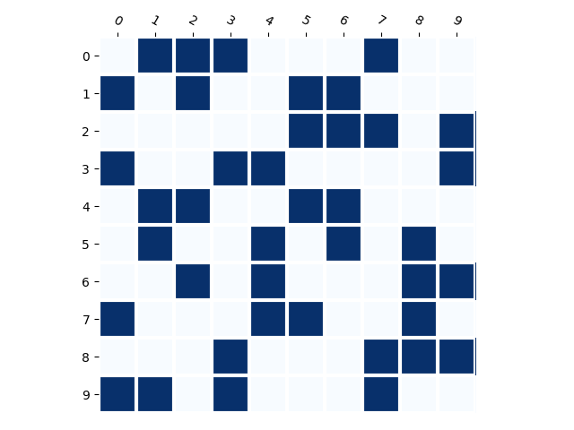
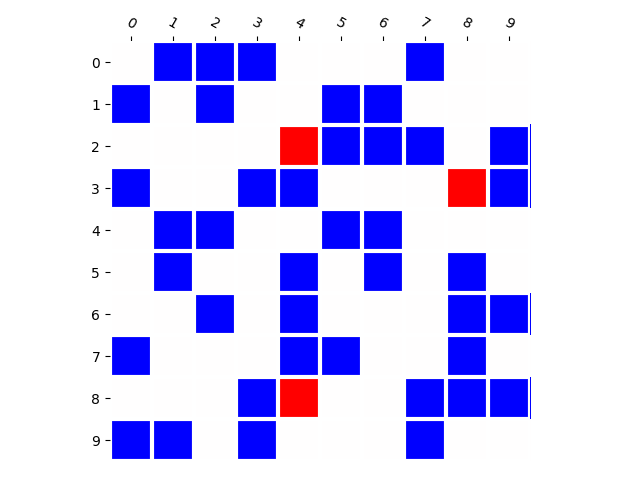
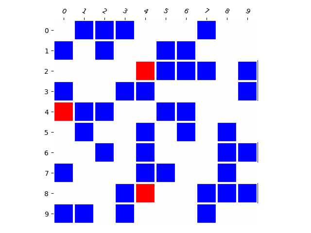
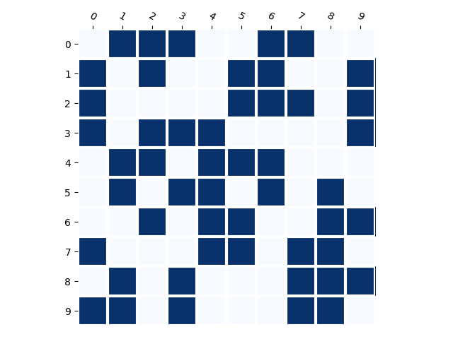
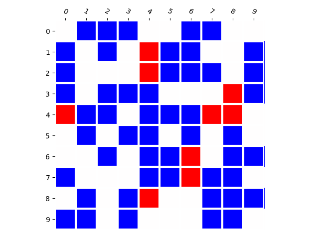
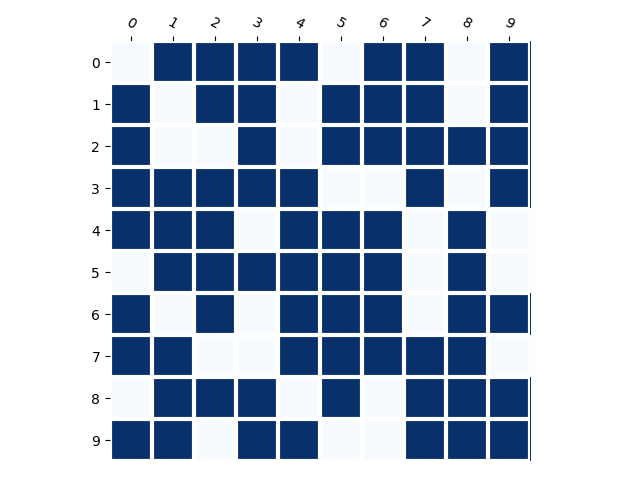
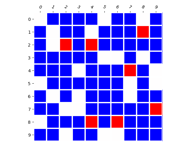
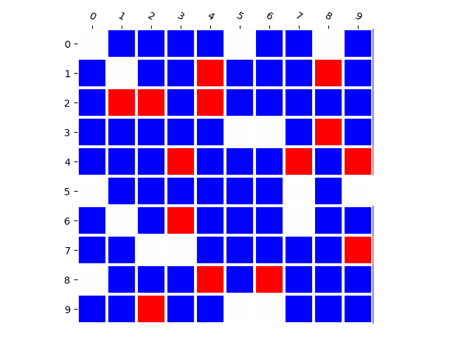
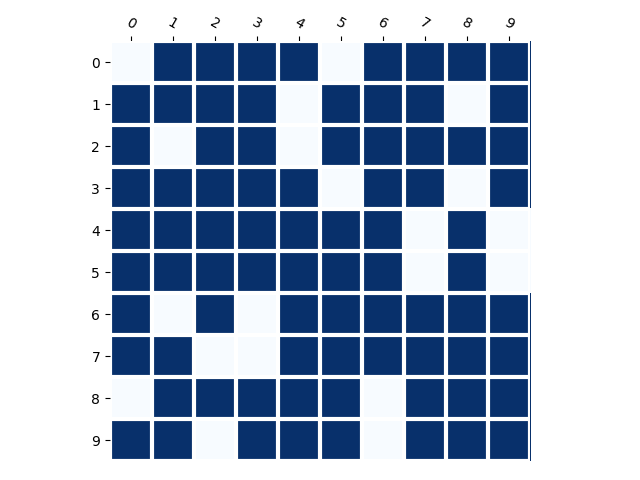
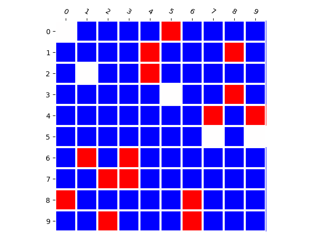
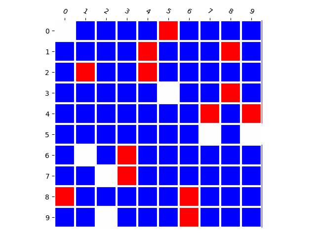
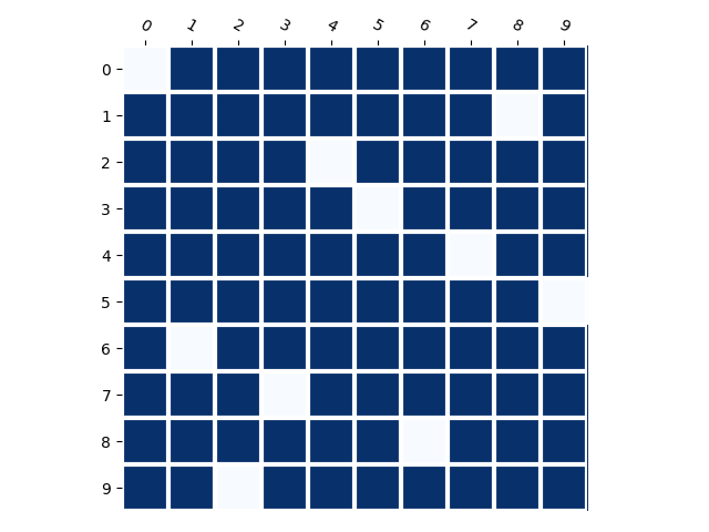
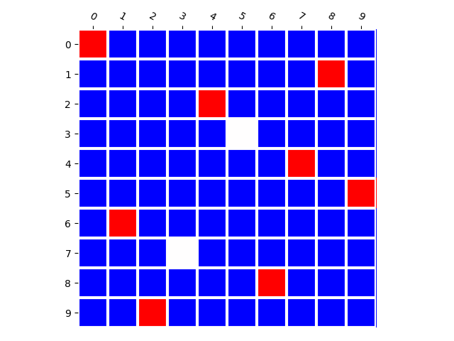
Below we visualize the input combinations (two MNIST digits, only some number combinations appear in the training set) compared to the output combinations. It can be observed that when there are few combinations (e.g. 10), the model does not generate much new combinations. When there are more (e.g. 80), the model generates almost every combination.
We emphasize that this is almost independent of model parameter-count and training set size. In fact, deep networks should be able to memorize huge amounts of random information [6], and when we train the model to classify which combinations appear in the training set by supervised training, it achieves perfect accuracy. This means that this phenomenon is closely related to how generative models are learned.
We believe that this property — whether generative models produce novel combinations — is particularly important. Therefore, we provide a toolbox to visualize this property, and to calculate a performance metric indicating whether the model is prone to memorization or prone to generalization.
References
[1] Deng, Jia, Wei Dong, Richard Socher, Li-Jia Li, Kai Li, and Li Fei-Fei. “Imagenet: A large-scale hierarchical image database.” In 2009 IEEE conference on computer vision and pattern recognition, pp. 248-255. Ieee, 2009.
[2] Brock, Andrew, Jeff Donahue, and Karen Simonyan. “Large scale gan training for high fidelity natural image synthesis.” arXiv preprint arXiv:1809.11096 (2018).
[3] Salimans, Tim, Andrej Karpathy, Xi Chen, and Diederik P. Kingma. “Pixelcnn++: Improving the pixelcnn with discretized logistic mixture likelihood and other modifications.” arXiv preprint arXiv:1701.05517 (2017).
[4] Kingma, Durk P., and Prafulla Dhariwal. “Glow: Generative flow with invertible 1x1 convolutions.” In Advances in Neural Information Processing Systems, pp. 10215-10224. 2018.
[5] Smith, J. David, and John Paul Minda. “Distinguishing prototype-based and exemplar-based processes in dot-pattern category learning.” Journal of Experimental Psychology: Learning, Memory, and Cognition 28, no. 4 (2002): 800.
[6] Zhang, Chiyuan, Samy Bengio, Moritz Hardt, Benjamin Recht, and Oriol Vinyals. “Understanding deep learning requires rethinking generalization.” arXiv preprint arXiv:1611.03530 (2016).
