TL;DR: Highlights from our AAAI 2018 paper, “Approximate Inference via Weighted Rademacher Complexity.” In this work we consider the challenging problem of computing the sum of more numbers than can be explicitly enumerated. This sum arises in various contexts, such as the partition function of a graphical model, the permanent of a matrix, or the number of satisfying assignments of a propositional formula. We show how this sum can be estimated and bounded by solving an optimization problem; finding the largest number in the sum after random perturbations have been applied.

Inference

Computing discrete integrals, or the sum of many numbers, is a basic task that is required for probabilistic inference in statistics, machine learning, and artificial intelligence. For example, Bayesian inference is used to predict the probability of a future event given past observations and a class of hypotheses, each specifying a probability distribution over events. In general the computation of a (discrete) integral is required for the calculation of posterior, marginal, or conditional distributions.

As an example, consider the distribution \(p(X_1, X_2)\) over two dependent binary random variables, \(X_1\) and \(X_2\). The marginal distribution \(p(X_1)\) is computed by summing the joint distribution over all values that \(X_2\) can take,

This is an easy calculation, but now consider the distribution \(p'(X_1, X_2, \dots, X_n)\) over \(n\) dependent binary random variables. Computing the marginal distribution

now requires summing \(2^{n-1}\) numbers, which will quickly become computationally intractable as \(n\) grows. Marginalizing just forty binary variables requires summing more than one trillion numbers. This exponential growth motivates us to look for approximations. To gain intuition into possible approaches, we first consider the simplest form of integration: counting.

Counting

To formalize the set counting problem, let’s define the set \(A\) as a subset of another set containing \(2^n\) elements, i.e. \(A \subseteq \{-1,1\}^n\) where each of the \(2^n\) elements is represented as a binary vector of length \(n\). We’re using \(-1\) and \(1\) as binary digits instead of \(0\) and \(1\) for reasons that will become clear later. Every element that belongs to \(A\) is given a weight of 1, that is \(w(\mathbf{x}) = 1\) for all \(\textbf{x} \in A\), while the remaining elements are given weight 0. Counting the number of elements in \(A\) is equivalent to summing all \(2^n\) weights, \(\sum_{\mathbf{x} \in \{-1,1\}^n} w(\mathbf{x}) = \left\vert{A}\right\vert\). Here’s an illustration of the counting problem, where we want to count the number of blue dots (\(\left\vert{A}\right\vert\)) that belong to the set of all \(2^n\) orange and blue dots.

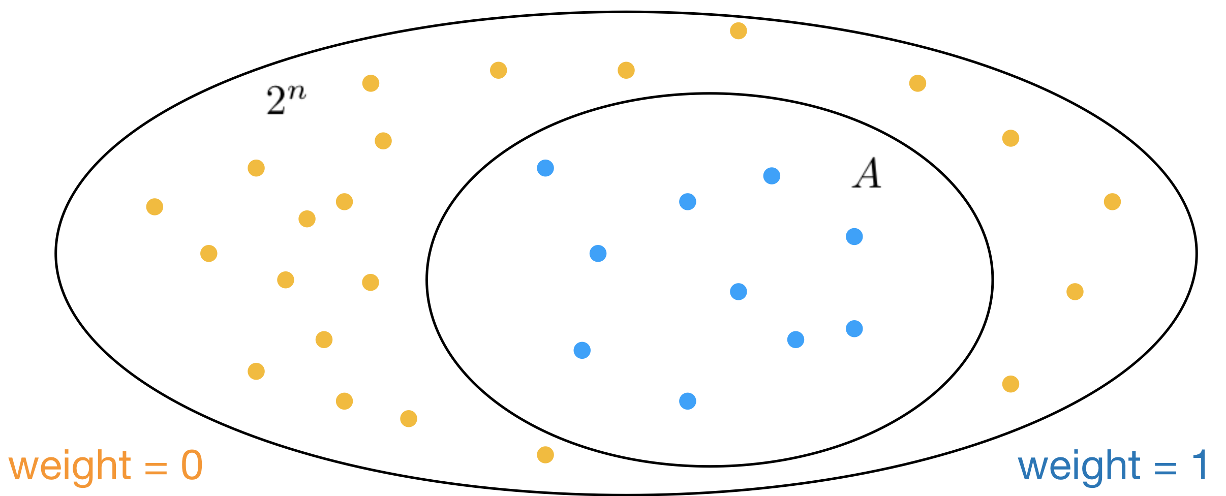
This particular problem is actually quite easy to solve, there are 10 blue dots. However \(n=5\) in this toy example and the problem will become exponentially more difficult as \(n\) increases.

In addition to being a small example, the above counting problem is particularly easy because the set \(A\) is structured and all its elements are in the same region of space. In general we cannot assume anything about the structure of \(A\). For instance the blue dots might just as well be scattered in space like this:

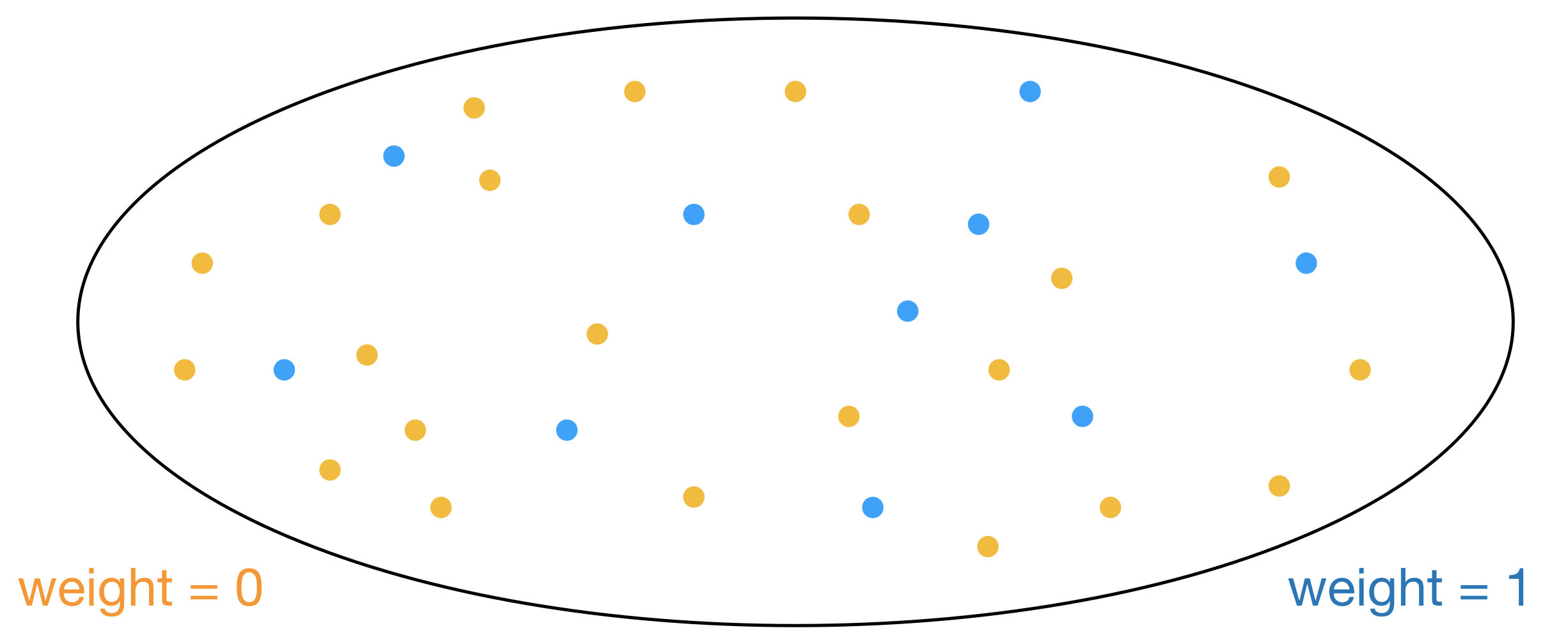
When the problem is totally unstructured counting requires enumeration of all \(2^n\) elements, checking whether each belongs to \(A\). This approach is not practical since the number of elements to enumerate grows exponentially.

This problem may seem contrived. How is it possible to create a set with \(2^{300}\) elements when the universe doesn’t even contain this many atoms? The answer is that sets can be defined implicitly as in the case of propositional model counting. In this case the set \(A\) is defined as all assignments to \(n\) binary variables that satisfy a boolean formula. Problems of this form motivate us to consider sets of size \(2^n\) because there are \(2^n\) possible assignments to \(n\) binary variables.

Summation

Computing the sum of a set of numbers (also referred to as discrete integration), is closely related to the counting problem. In fact summation is a more general problem; if each number in the set is defined to be 1 then summation is equivalent to counting.

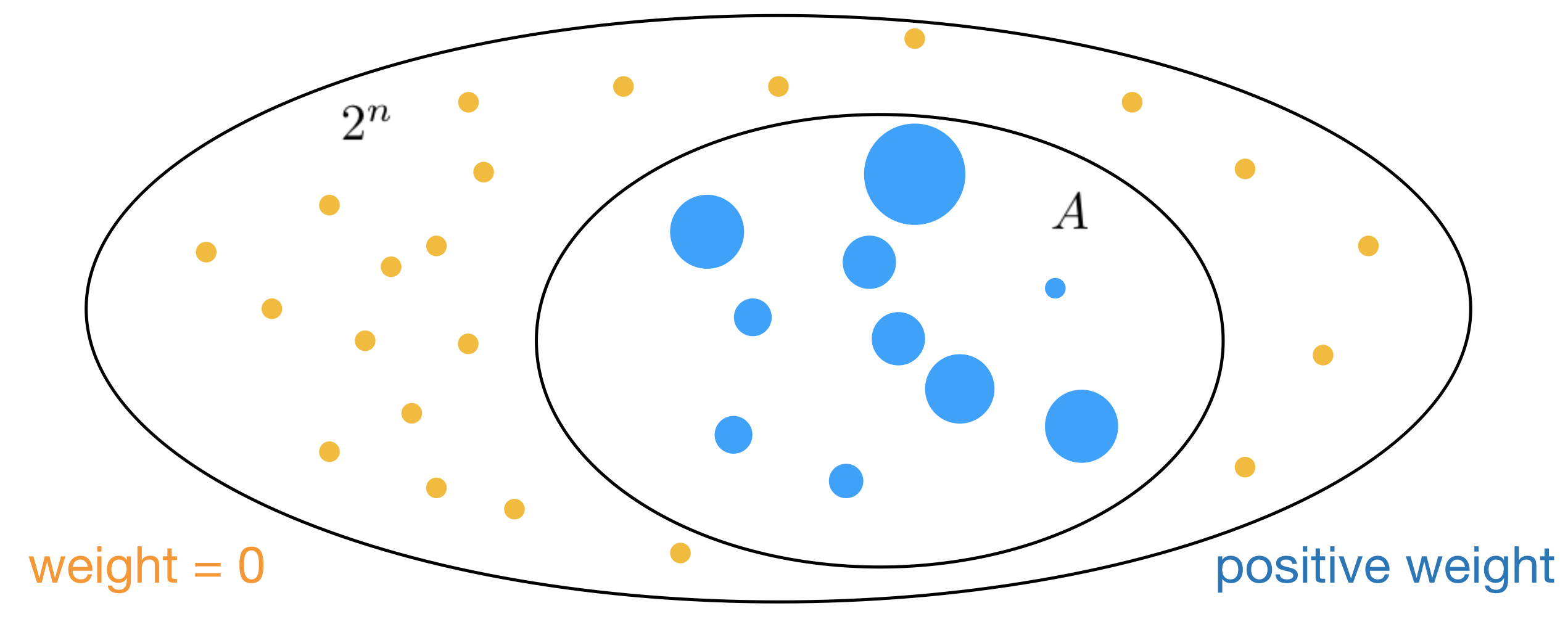
Formally, we can keep our definition of \(A\) as some subset of another set containing \(2^n\) elements, \(A \subseteq \{-1,1\}^n\). Every element that belongs to \(A\) is still given a weight, but now this weight may be any positive number (\(w(\mathbf{x}) > 0\), for \(\textbf{x} \in A\)), while the remaining elements are given weight 0. The sum of weights, \(\sum_{\mathbf{x} \in \{-1,1\}^n} w(\mathbf{x}\)), can be viewed as the weighted set size. Below is an illustration of a weighted set, where the sizes of blue dots represent weights:

Rademacher Complexity

The number of elements contained in a set can be viewed as a measure of the set’s complexity. The notion of complexity arises in a variety of fields under various forms. In statistical mechanics the concept of entropy is closely linked to set size. The Kolmogorov complexity is defined as the shortest computer program that can produce an object in the field of information theory. VC dimension and Rademacher Complexity are used in computational learning theory to guarantee the performance of a learned hypothesis on unseen test data, based on the complexity of the set of hypotheses it was selected from. Rademacher complexity is defined in terms of how well the hypothesis class can fit random noise. These notions of complexity are each affected differently by structure in the set space and none is fundamentally the best; whether figurative paintings such as the Mona Lisa or abstract paintings like No. 5 are more complex is a rather philosophical question. While each measure of complexity treats structure differently, they are also related. For example, a large set with many elements will typically require a long program to be described (Kolmogorov complexity). Here, we focus on the relationship between Rademacher complexity and set size.

The Rademacher complexity of a set \(A \subseteq \mathbb{R}^n\) is defined as

where \(\mathbf{c}\) is sampled uniformly from \(\{-1, 1\}^n\), \(\mathbb{E}_{\mathbf{c}}\) denotes an expectation over \(\mathbf{c}\), and sup is short for supremum (which we may consider to be the maximum). It may seem peculiar to define such a quantity in terms of a randomly sampled vector, but it turns out that randomness is a surprisingly powerful tool for computing difficult quantities. For instance, \(\pi\) can be calculated by randomly dropping needles on a hardwood floor with evenly spaced lines.

Intuition

The expression \(\sum_{i=1}^n c_i a_i\) is a dot product between vectors \(\mathbf{c}\) and \(\mathbf{a}\), which measures how close the direction of \(\mathbf{c}\) is to \(\mathbf{a}\). To visualize the Rademacher complexity let’s map all \(n\)-dimenional vectors in \(A\) to a 2-dimensional circle:

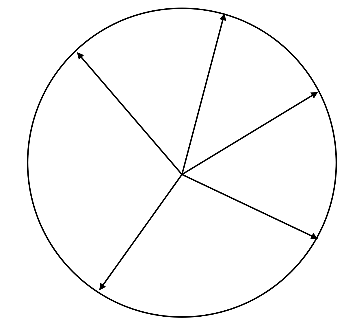
Calculating the Rademacher complexity now requires the following steps:

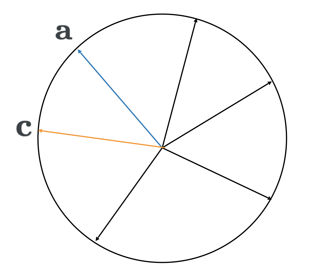
1. Sample a random vector \(\mathbf{c}\)

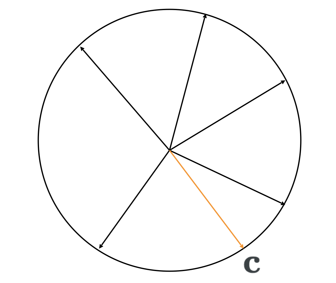
2. Find the vector \(\mathbf{a}\) that has the largest dot product with \(\mathbf{c}\), from among all vectors in set \(A\)

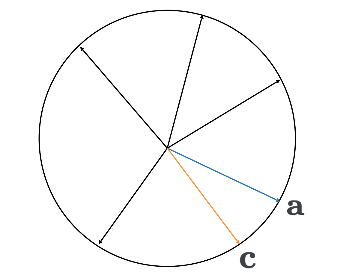
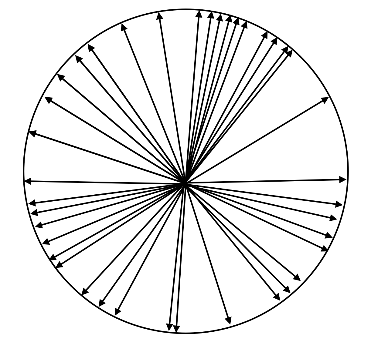
3. Repeat steps one and two an exponential number of times to enumerate maximum dot products with all \(2^n\) possible vectors \(\mathbf{c}\)

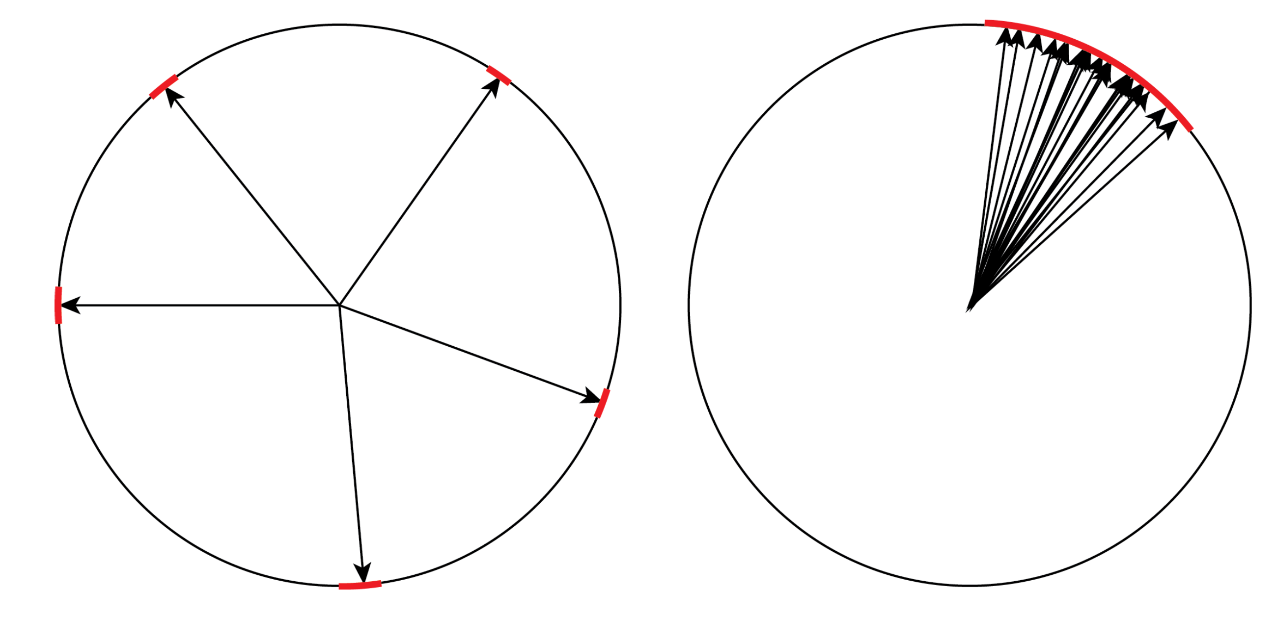
One snag with the above procedure for calculating the Rademacher complexity is that step three requires an exponential number of repetitions (for every possible value of \(c\)). Fortunately, Rademacher complexity has the nice property of being concentrated. This means that an estimate obtained by only repeating steps one and two a small number of times can be guaranteed to be good with high probability using concentration inequalities.

Quantitative Relationships

Generally, small sets like the one above will have a small Rademacher complexity because there are few regions of space where a random vector would have a large dot product with any vector in the set. On the other hand, very large sets generally have large Rademacher complexities because most regions of space where a random vector could be sampled have a large dot product with some vector in the set:

Adding vectors to a set increases its Rademacher complexity.

Can we formalize this intuition? Quantitative relationships between Rademacher complexity and size of a hypothesis class are widely used in learning theory. Massart’s Lemma upper bounds the Rademacher complexity of a set in terms of the set’s size, regardless of the set’s structure. In other words, Massart’s Lemma formally guarantees that the Rademacher complexity of a set will be smaller than some function of the set’s size. This is useful in learning theory where proving that the Rademacher complexity of a hypothesis class is small can be used to show that a hypothesis learned from training data will generalize well to unseen test data. The proof of Massart’s Lemma depends on the fact that the maximum is never greater than the sum of a set of numbers.¹

Unfortunately, the same trick won’t work to lower bound the Rademacher complexity in terms of set size (we can’t say that the maximum element in a set is greater or equal to the sum of elements, unless the set only contains one non-zero element, which isn’t an interesting case). Alexander Barvinok developed a proof technique to lower bound the solution to a randomly perturbed optimization problem in terms of set size (Barvinok 1997). We discovered that the solution to his optimization problem is in fact the Rademacher complexity, which allows us to provide both upper and lower bounds on the Rademacher complexity in terms of set size.²

Armed with both upper and lower bounds we can estimate the size of a set given its Rademacher complexity. The key insight is that Rademacher complexity can be efficiently estimated for a class of interesting problems, even though computing set size is intractable due to the possibly exponential number of elements. This depends on the fact that Rademacher complexity is defined in terms of an optimization problem rather than a sum.

Optimization

Even though computing the sum of all elements in a very large set is intractable, finding the largest element is easy in many cases. For example, consider all buildings in New York City and their associated heights. Viewing each building as an element in a set, building heights correspond to element weights. Computing the sum of all weights, \(\sum_{\mathbf{x} \in \{-1,1\}^n} w(\mathbf{x}\)), would require measuring the height of each building in New York and adding up all the recorded heights.

In contrast, finding the height of the tallest building is an easy task.

From a distance it’s clear that One World Trade Center is the tallest building in New York, leaving us to measure the height of only a single building. Operations research, optimization, and related fields have produced a huge selection of literature on methods including branch and bound and techniques for relaxation that exploit this intuition.

Our approach to computing intractable sums is to solve an optimization problem where we find the largest element in a set. This approach doesn’t sound promising. For instance, the sum of the numbers 1,2,3…,100 is 5,050 (\(101\times50\)), but the largest number in the set is 100 which is too small by over a factor of 50. To improve on this idea we will use the power of randomized algorithms.

Weighted Rademacher Complexity

In the previous section we discussed the relationship between two notions of complexity, set size and Rademacher complexity. This relationship makes it possible to estimate set size using Rademacher complexity, turning the counting problem into the problem of calculating the Rademacher complexity, which is an optimization problem. Whenever the corresponding optimization problem can be solved efficiently, this can be an effective strategy.

However, in many applications we are interested in the more complicated problem of calculating arbitrary sums of non-negative numbers (e.g., probabilities), or weighted set sizes. How can we adapt the previous strategy to this more general case?

To do this we introduce the weighted Rademacher complexity,

of weight function \(w:\{-1,1\}^n \rightarrow [0, \infty)\) (which can be viewed as a weighted set). Note that we still sample \(\mathbf{c}\) uniformly from \(\{-1, 1\}^n\) and \(\langle \mathbf{c},\mathbf{x} \rangle\) is the dot product between vectors \(\mathbf{c}\) and \(\mathbf{x}\). The weighted Rademacher complexity of a weighted set is analogous to the Rademacher complexity of an unweighted set.

Calculating the weighted Rademacher complexity of \(w\) exactly requires solving \(2^n\) optimization problems, as in the unweighted case. Now the optimization problems have been modified and require finding the logarithm of the largest weight, \(\log w(x)\), subject to random perturbations. The random perturbations to each log weight take the form of the quantity optimized in the unweighted setting; the dot product of a randomly sampled vector with the weight’s location vector, \(\langle \mathbf{c},\mathbf{x} \rangle\).

Intuition

As intuition for our construction of the weighted Rademacher complexity, we maintain two desirable properties. For an indicator weight function that only takes values of 0 or 1 we recover the standard Rademacher complexity. For \(m\)-dimensional, hypercube shaped weight functions that take only the values 0 and \(a\), the weighted Rademacher complexity is an unbiased estimator of \(\log_2\) of the weighted set size, which is \(m + \log_2 a\).

We proved that the weighted Rademacher complexity can be bounded by the weighted set size, \(\sum_{\mathbf{x} \in \{-1,1\}^n} w(\mathbf{x}\)). Our upper bound is a generalization of Massart’s Lemma to the weighted setting. Our approach to proving the lower bound is inspired by Barvinok. The proof is recursive and implicitly divides the weight function in half at each step, maintaining a relationship between weighted Rademacher complexity and weighted set size. Additionally, we account for the value of the single weight we are left with after dividing the space \(n\) times. We show the weighted Rademacher complexity is concentrated using McDiarmid’s inequality, which allows us to develop an efficient algorithm.

Developing an Algorithm

The weighted Rademacher complexity can be estimated by solving a small number of randomly perturbed optimization problems of the form

where \(\mathbf{c}\) is sampled uniformly from \(\{-1, 1\}^n\). This perturbation has the advantageous property that for any log-supermodular weight function, where the largest weight can be found efficiently, the perturbed optimization problem can also be solved efficiently (Bach and others 2013).

We can get away with estimating the expectation using only a small number of samples because we showed the weighted Rademacher complexity is concentrated. This means we can state that with high probability the weighted Rademacher complexity is within some bound of our estimate. Combining our concentration bound with upper and lower bounds on the Rademacher complexity of a set in terms of the set’s size, we give bounds that hold with high probability on the weighted set size in terms of solutions to a small number of optimization problems.

Discussion

It is interesting to note that the weighted Rademacher complexity has nearly the same form as the Gumbel-max trick (Papandreou and Yuille 2011; Hazan and Jaakkola 2012). Replacing the vector \(\mathbf{c}\) of Rademacher variables with independent and identically distributed Gumbel variables (\(\gamma(\mathbf{x})\)) we have the Gumbel-max trick

In this light the Gumbel-max trick may be viewed as another complexity, which gives an unbiased estimate of the weighted set size. We experimentally compared our method with a low-dimensional Gumbel perturbation based method, finding that we were able to produce tighter bounds on a variety of problems given limited computation (please refer to our paper for further details).

Another related line of work uses randomized hashing schemes to approximate weighted set size (Ermon et al. 2013). These approaches also solve randomly perturbed optimization problems to compute their bounds. Randomized hashing based methods can find much tighter bounds than ours in some settings, but as a trade-off require random perturbations that make the resulting optimization problems much more computationally expensive to solve.

Worst Case Scenarios

While there is a general relationship between Rademacher complexity and set size, it can be loose because the Rademacher complexity also depends on the set’s shape. A small but uniformly distributed set can have the same Rademacher complexity as a relatively large but tightly packed set. When a small set is uniformly distributed through space a randomly chosen vector can have a large dot product with at most one vector in the set. However, for a tightly packed set, the regions of space corresponding to a large dot product with each vector in the set will overlap, so that the total region which has a large dot product with any vector in the set will remain small as illustrated below (where red corresponds to regions of space that have a large dot product with at least one vector in the set):

These two sets describe worst case scenarios, which our bounds must take into account. This places a fundamental limit on how tight our bounds can be.

Future Work

Noting the similarity between the weighted Rademacher complexity and Gumbel-max trick, in the future weighted Rademacher complexity may be generalized to other forms of randomness.

In the context of learning theory, Rademacher complexity measures how well a hypothesis class can fit random noise. As more hypotheses are added to a class, the class becomes more capable of fitting random noise and also more complex. Similarly, the weighted Rademacher complexity is a measure of how well a hypothesis class can fit random noise using Bayesian inference, given a prior probability distribution over hypotheses. In this setting the prior over hypotheses, in addition to the actual hypotheses present in the class, affects the complexity of the class. A uniform prior over hypotheses (reflecting uncertainty in prior belief) will make it easier to fit random noise. The same hypothesis class, but with a prior that assigns high probability to only a few hypotheses, will not fit random noise as well making the class less complex. The weighted Rademacher complexity reflects these properties. In the future, this new definition for the complexity of a hypothesis class in the context of Bayesian inference could be used to derive bounds on learnability and generalization error.

Approximate Inference via Weighted Rademacher Complexity
Jonathan Kuck, Ashish Sabharwal, Stefano Ermon
AAAI Conference on Artificial Intelligence, 2018.
paper code

Footnotes

References

1. Barvinok, Alexander I. 1997. “Approximate Counting via Random Optimization.” Random Structures and Algorithms 11 (2): 187–98.
2. Bach, Francis, and others. 2013. “Learning with Submodular Functions: A Convex Optimization Perspective.” Foundations and Trends in Machine Learning 6 (2-3): 145–373.
3. Papandreou, George, and Alan L Yuille. 2011. “Perturb-and-Map Random Fields: Using Discrete Optimization to Learn and Sample from Energy Models.” In Computer Vision (ICCV), 2011 IEEE International Conference On, 193–200. IEEE.
4. Hazan, Tamir, and Tommi S. Jaakkola. 2012. “On the Partition Function and Random Maximum A-Posteriori Perturbations.” In Proceedings of the 29th International Conference on Machine Learning (ICML-12), 991–98. ACM.
5. Ermon, Stefano, Carla Gomes, Ashish Sabharwal, and Bart Selman. 2013. “Taming the Curse of Dimensionality: Discrete Integration by Hashing and Optimization.” In Proceedings of the 30th International Conference on Machine Learning (ICML-13), 334–42.