Reflected Diffusion Models
Introduction
Diffusion models are a new class of generative models which have quickly supplanted traditional models like GANs, VAEs, and Normalizing Flows in many domains such as image, language, and molecule generation. They have also been the driving force behind several famous text-to-image generation systems like DALLE-2, Imagen, and Stable Diffusion.
At their core, diffusion models start by perturbing data on \(\mathbb{R}^d\) with a hand-designed “forward” stochastic differential equation (SDE) with fixed coefficients \(\mathbf{f}\) and \(g\):
Forward process. Image courtesy of Yang Song.
\[\begin{equation} \mathrm{d} \mathbf{x}_t = \mathbf{f}(\mathbf{x}_t, t) \mathrm{d}t + g(t) \mathrm{d} \mathbf{B}_t \end{equation}\]taking our initial data distribution \(p_0\) to a stationary distribution $p_T$ (normally a simple distribution like a Gaussian). Using time reversed Brownian motion \(\overline{\mathbf{B}}_t\) and the score function \(\nabla_x \log p_t\), one can construct a corresponding “reverse” SDE which takes \(p_T\) to \(p_0\):
Reverse process. Image courtesy of Yang Song.
\[\begin{equation} \mathrm{d} \mathbf{x}_t = \left[\mathbf{f}(\mathbf{x}_t, t) - g(t)^2 \nabla_x \log p_t(\mathbf{x}_t) \right]\mathrm{d}t + g(t) \mathrm{d} \overline{\mathbf{B}}_t \end{equation}\]This defines a stochastic transport from our simple distribution $p_T$ to our data distribution $p_0$, so we can build a generative model by approximating this process.
The only unknown component is the score function \(\nabla_x \log p_t\), which can be learned with a time-dependent score neural network \(\mathbf{s}_\theta(\mathbf{x}, t)\). To train, we optimize what is known as the score matching loss:
\[\begin{equation} \mathbb{E}_{t \in [0, T]} \mathbb{E}_{\mathbf{x} \sim p_t} \ \lambda_t \| \mathbf{s}_\theta(\mathbf{x}_t, t) - \nabla_x \log p_t(\mathbf{x}_t)\|^2 \end{equation}\]Here, $\lambda_t$ is a weighting function that alters the final models behavior. For example, setting \(\lambda_t = g(t)^2\) maximizes the log-likelihood of the generated data, and setting \(\lambda_t = 1 /\mathbb{E}\|\nabla_x \log p_t(x_t \vert x_0)\|^2\) improves image quality. Once we learn \(\mathbf{s}_\theta\), we can generate samples from our diffusion model by first sampling \(\mathbf{x}_T \sim p_T\) and solving the reverse SDE from \(T\) to \(0\):
\[\begin{equation} \mathrm{d} \mathbf{x}_t = \left[\mathbf{f}(\mathbf{x}_t, t) - g(t)^2 s_\theta(\mathbf{x}_t, t) \right]\mathrm{d}t + g(t) \mathrm{d} \overline{\mathbf{B}}_t \end{equation}\]Thresholding
Unfortunately, the devil always lies in the details. We need to discretize time to simulate the generative SDE, resulting in an Euler-Maruyama scheme with i.i.d. Brownian increments \(\mathbf{B}_{\Delta t}^t \sim \mathcal{N}(0, \Delta t)\):
\[\begin{equation} \mathbf{x}_{t - \Delta t} = \mathbf{x}_{t} - \left[\mathbf{f}(\mathbf{x}_t, t) - g(t)^2 s_\theta(\mathbf{x}_t, t) \right] \Delta t + g(t) \mathbf{B}_{\Delta t}^t \end{equation}\]Numerical error can arise from the discretization, the learned score function, or just plain bad luck when sampling the increments, causing our trajectory \(\mathbf{x}_t\) to enter low probability regions. Since we train with the Monte Carlo version of our loss
\[\begin{equation} \frac{1}{nm} \sum_{i = 1}^{n} \sum_{j = 1}^m \ \lambda_{t_i} \| \mathbf{s}_\theta(\mathbf{x}_{t_i}^j, t_i) - \nabla_x \log p_{t_i}(\mathbf{x}_{t_i}^j)\|^2 \end{equation}\]it is even possible to never optimize in low probability regions, so the score network behavior there tends to be undefined. Previously, this problem appeared for vanilla score matching, degrading the performance of naive Langevin dynamics. For diffusion models, this problem again resurfaces, this time as a compounding error in the sampling process. For a lot of cases, this causes samples to drastically diverge, leading to obviously wrong blank images:

Sampling from Diffusion Models beat GANs on Image Synthesis with ‘clip_denoised=False’.
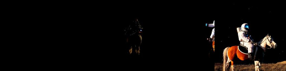
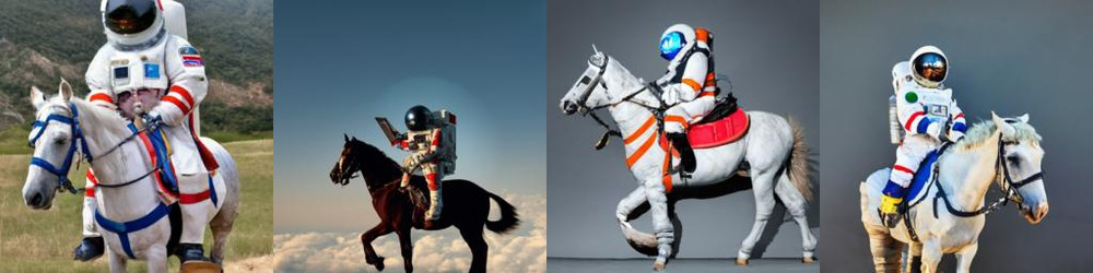
Divergent samples originally reported in Imagen. ‘An astronaut riding a horse’.
Diffusion models were initially motivated as a stack of VAEs which gradually denoised the input. The Euler-Maruyama step can be decomposed based on this perspective:
\[\begin{equation} \mathbf{x}_{t - \Delta t} = \underbrace{\mathbf{x}_{t} - \left[\mathbf{f}(\mathbf{x}_t, t) - g(t)^2 s_\theta(\mathbf{x}_t, t) \right] \Delta t}_{\text{VAE Predicted Mean } \overline{\mathbf{x}}_{t - \Delta t}} + \underbrace{g(t) \mathbf{B}_{\Delta t}^t}_{\text{VAE Noise}} \end{equation}\]inspiring a natural fix. We seek to generate images, so the predicted mean \(\overline{\mathbf{x}}_{t - \Delta t}\) should be a “valid” image. This can be accomplished by clipping each pixel to the fixed \([0, 255]\) range (which can be rescaled to \([0, 1]\) or \([-1, 1]\) depending on the context), and this trick is known as thresholding. You can find many examples of it in the repositories of famous papers, although it is almost never mentioned:
Thresholding avoids the divergent behavior we saw previously, generating much nicer samples.

Sampling from Diffusion Models beat GANs on Image Synthesis with ‘clip_denoised=True’.
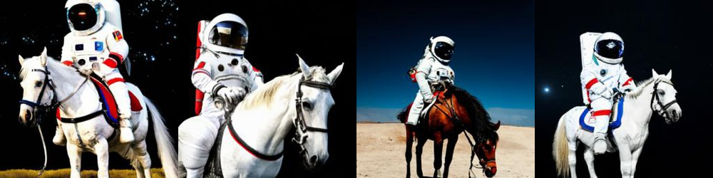
Thresholded samples originally reported in Imagen. ‘An astronaut riding a horse’. These are quite saturated.
Unfortunately, diffusion models are supposed to reverse the forward corrupting process. Changing the generative process like this breaks the fundamental assumption, resulting in a mismatch. This has been linked with phenomena like oversaturation when using a large amount of diffusion guidance (such as in the Imagen generated example), necessitating task-specific techniques that don’t generalize, such as dynamic thresholding
Dynamically thresholded samples originally reported in Imagen. ‘An astronaut riding a horse’.
Reflected Diffusion Models
As we take \(\Delta t \to 0\), the thresholded Euler Maruyama scheme
\[\begin{equation} \mathbf{x}_{t + \Delta t} = \mathrm{proj}\left(\mathbf{x}_{t} + \mathbf{f}(\mathbf{x}_t, t) \Delta t\right) + g(t) \mathbf{B}_{\Delta t}^t \end{equation}\]converges to what’s known as a reflected stochastic differential equation:
\[\begin{equation} \mathrm{d} \mathbf{x}_t = \mathbf{f}(\mathbf{x}_t, t) \mathrm{d}t + g(t) \mathrm{d} \mathbf{B}_t + \mathrm{d} \mathbf{L}_t \end{equation}\]The behavior is exactly the same on the interior of our domain, but, at the boundary, the new term \(\mathbf{L}_t\) “zeroes out” all outward pointing force to ensure the particle stays within the constraints.

Reflected Brownian Motion, the canonical example of a reflected SDE. The process will never go below 0.
Similar to standard stochastic differential equations, it is possible to reverse this with a reverse reflected stochastic differential equation
\[\begin{equation} \mathrm{d} \mathbf{x}_t = \left[\mathbf{f}(\mathbf{x}_t, t) - g(t)^2 \nabla_x \log p_t \right]\mathrm{d}t + g(t) \mathrm{d} \overline{\mathbf{B}}_t + \mathrm{d} \overline{\mathbf{L}}_t \end{equation}\]This forms the same forward/reverse coupling that undergirds standard diffusion models, so we can use this principle to define Reflected Diffusion Models.
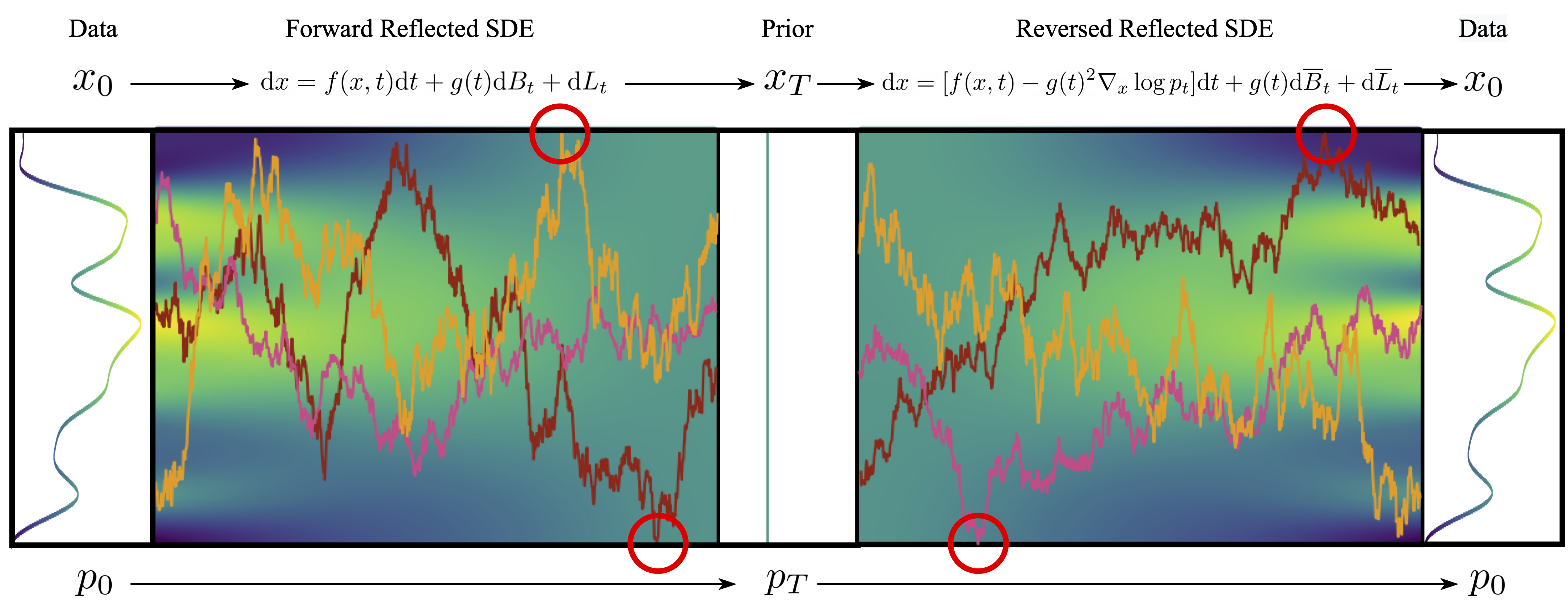
An overview of reflected diffusion models. We learn to reverse a reflected stochastic differential equation.
Score Matching on Bounded Domains
To construct our Reflected Diffusion Models, we need to learn \(\nabla_x \log p_t\). These are the marginal scores recovered from the forward reflected SDE, not the standard forward SDE. The score matching loss can be made more tractable by employing the denoising trick from standard diffusion models, reducing our loss to a (weighted combination) of denoising score matching losses for each \(p_t\)
\[\begin{equation} \mathbb{E}_{\mathbf{x} \sim p_0} \mathbb{E}_{\mathbf{x}_t \sim p_t(\cdot \vert x_0)} \| \mathbf{s}_\theta(\mathbf{x}_t, t) - \nabla_x \log p_t(\mathbf{x}_t | \mathbf{x}_0)\|^2 \end{equation}\]One still needs to accurately compute the transition density \(p_t(\mathbf{x}_t \vert \mathbf{x}_0)\) quickly, which is not available in closed form. In particular, \(p_t(\mathbf{x}_t \vert \mathbf{x}_0)\) is actually a reflected Gaussian variable, and this leads to two natural computation strategies:
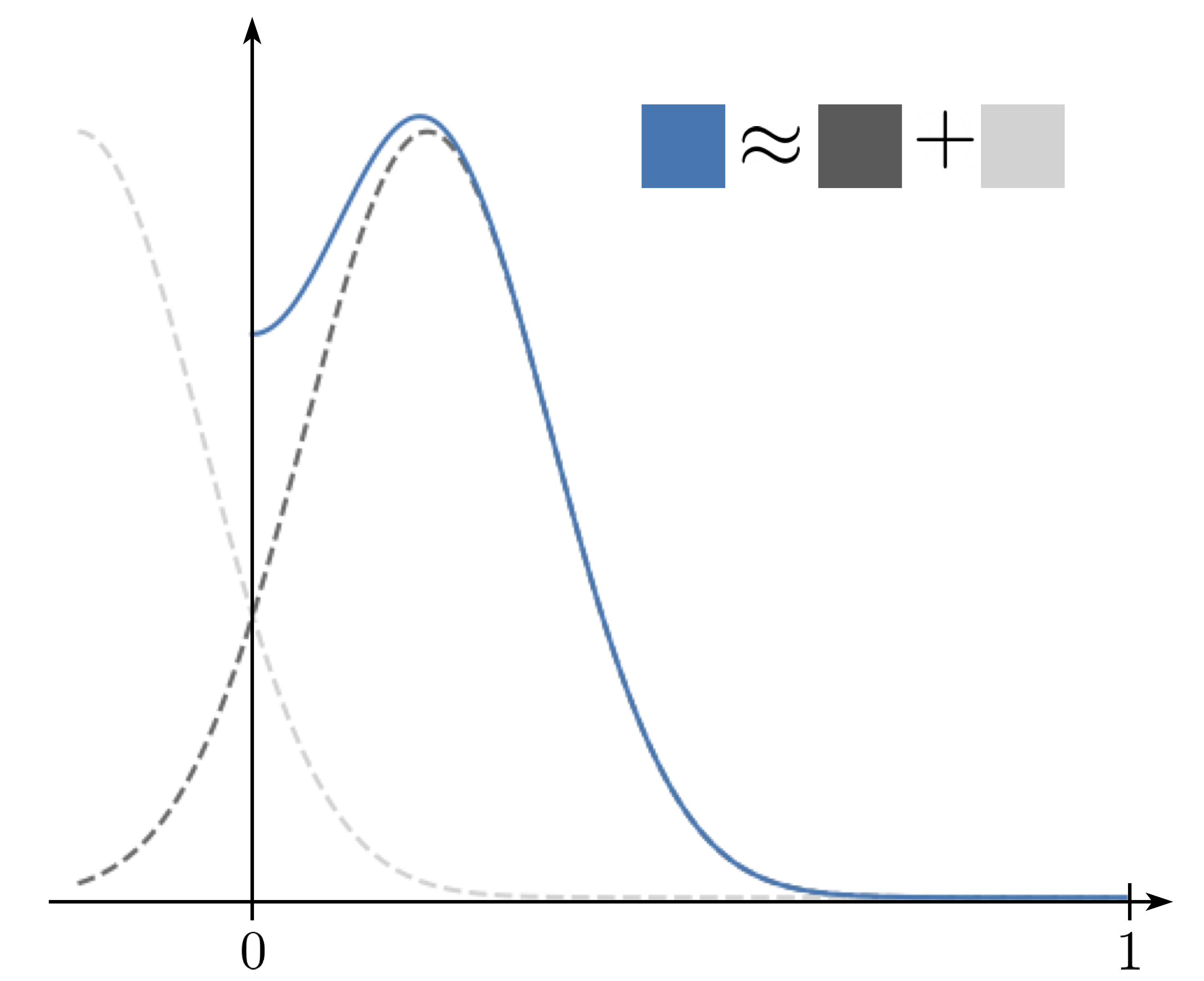
Strategy 1: sum up all of the reflected components of the Gaussian.
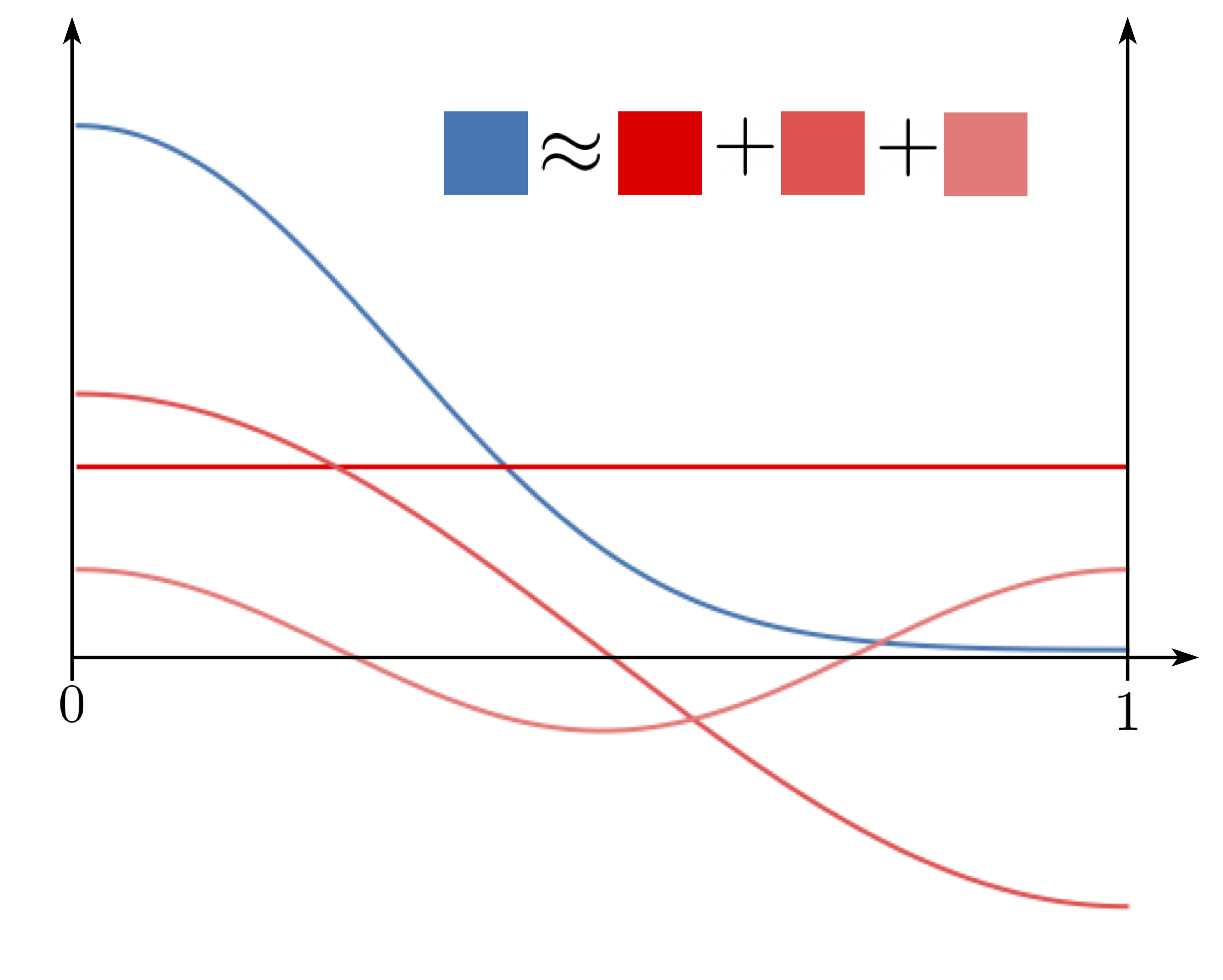
Strategy 2: decompose the distribution using harmonic analysis.
Strategy 1 is accurate for small times since we don’t need to compute as many reflections, while strategy 2 is accurate for large times since the distribution goes closer to uniform, requiring fewer harmonic components. These strategies shore up the other’s weaknesses, so we combine them to efficiently compute the transition density.
How to Solve Reverse Reflected SDEs
We have already seen that thresholding provides a Euler-Maruyama type discretization. The core idea is that it approximates \(\mathbf{L}_t\) in discrete time. However, we are by no means limited to just thresholding. We found that approximating the process with a reflection term produced better samples:
\[\begin{equation} \mathbf{x}_{t - \Delta t} = \mathrm{refl}\left(\mathbf{x}_{t} - \left[\mathbf{f}(\mathbf{x}_t, t) - g(t)^2 \mathbf{s}_\theta(\mathbf{x}_t, t) \right] \Delta t + g(t) \mathbf{B}_{\Delta t}^t\right) \end{equation}\]This produces reasonable samples, but we can actually further augment the sampling procedure. Since \(\mathbf{x}_t \sim p_t\), we can use our score function to define a predictor-corrector update scheme based on Constrained Langevin Dynamics to “correct” our sample \(\mathbf{x}_t\):
\[\begin{equation} \mathrm{d} \mathbf{x}_t = \frac{1}{2} s_\theta(\mathbf{x}_t, t) \mathrm{d} t + \mathrm{d} \mathbf{B}_t + \mathbf{L}_t \end{equation}\]With this component, we match all of the constructs from standard diffusion models. We can achieve state-of-the-art perceptual quality (as measured by Inception score) without modifying the architecture or any other components. Unfortunately, the FID score, another common metric, tends to lag behind because our generated samples have noise (at the scale of 1-2 pixels) that FID is notoriously sentitive to.
| Method | Inception score (↑) |
|---|---|
| NCSN++ (Song et al. 2021) | 9.89 |
| Subspace Diffusion (Jing et al. 2022) | 9.99 |
| Ours | 10.42 |
Probability Flow ODE
Analogous to the widely used DDIM scheme, we can anneal our reflected SDE to a new noise level \(\overline{g}(t) > 0\).
\[\begin{equation} \mathrm{d} \mathbf{x}_t = \left[\mathbf{f}(\mathbf{x}_t, t) - \frac{g(t)^2 - \overline{g}(t)^2}{2} \nabla_x \log p_t(\mathbf{x}_t) \right] \mathrm{d}t + \overline{g}(t) \mathrm{d} \mathbf{B}_t + \mathrm{d} \mathbf{L}_t \end{equation}\]This results in a reflected diffusion process that has the same marginal probabilities as our original SDE, and allows us to sample with a lower variance. Amazingly, as we take \(\overline{g}(t) \to 0\), the boundary reflection term \(\mathrm{d} \mathbf{L}_t\) disappears since \(\nabla_x \log p_t\) satisfies Neumann boundary conditions:
\[\begin{equation} \mathrm{d} \mathbf{x}_t = \left[\mathbf{f}(\mathbf{x}_t, t) - \frac{g(t)^2}{2} \nabla_x \log p_t(\mathbf{x}_t)\right]\mathrm{d}t \end{equation}\]We can replace \(\nabla_x \log p_t\) with our score function approximation $\mathbf{s}_\theta$ to recover a Probability Flow ODE. This enables fast sampling with efficient ODE samplers, an interpretable latent space, and exact log-liklihoods through the Hutchinson trace estimator trick.
Interestingly, learning with the \(\lambda_t\) weighting function that we used for image generation results in an ELBO, so we can use the same noise schedule to generate good images and maximize likelihoods. When compared with other likelihood-based diffusion methods, our optimization has much lower variance, so we can achieve likelihood results that are close to the state of the art without requiring either importance sampling or a learned noise schedule.
| Method | CIFAR-10 BPD (↓) | ImageNet-32 BPD (↓) | |
|---|---|---|---|
| ScoreFlow (Song et al. 2021) | 2.86 | 3.83 | |
| (with importance sampling) | 2.83 | 3.76 | |
| VDM (Kingma et al. 2021) | 2.70 | —— | |
| (with learned noise) | 2.65 | 3.72 | |
| Ours | 2.68 | 3.74 |
Diffusion Guidance
One of the major perks of diffusion models is their controllability. Using some conditional information \(\mathbf{c}\), which could be the class or a piece of description text, we can guide samples to satisfy \(c\) through a classifier \(p(\mathbf{c} \vert \mathbf{x})\):
\[\begin{equation} \nabla \log p_t(\mathbf{x} \vert c) = \nabla \log p_t(\mathbf{x}) + \nabla \log p_t(c \vert \mathbf{x}) \end{equation}\]Currently, this notion of controllable diffusion normally appears as classifier-free diffusion guidance, which instead uses an additional conditional score network and a guidance weight \(w\) to approximate the synthetic distribution \(p_t^w(\mathbf{x} \vert c) \propto p_t(\mathbf{x}) p_t(c \vert \mathbf{x})^w\):
\[\begin{equation} \nabla \log p_t^w(\mathbf{x} \vert c) = (w + 1) \nabla \log p_t(\mathbf{x} \vert c) - w \nabla \log p_t(\mathbf{x}) \end{equation}\]In the literature, increasing \(w\) generates more fidelitous images, which is crucial for text-to-image guided diffusion. From our experiments, we found that thresholding is critical for classifier-free guidance to work. Without it, sampling with even small weights \(w\) causes images to diverge:

Baseline non-thresholded images for \(w=1\).
Additionally, we can’t use quick deterministic ODE sampling methods since we can’t mimic the effect of thresholding. In fact, this seems to cause samples to diverge even more:

Baseline non-thresholded images for \(w=1\). Sampled with an ODE.
Furthermore, although a large guidance weight \(w\) is preferred in applications such as text-to-image diffusion, it is well known that this can cause samples to suffer artifacts such as oversaturation even when thresholding.

Baseline thresholded images for \(w=15\). They suffer from oversaturation.
We hypothesize that this these artifacts are due to the mismatch between training and sampling. In particular, the trained behavior seeks to push samples out-of-bounds, and the sampling procedure clips these out-of-bounds pixels to \(0\) or \(255\), resulting in oversaturation. Because Reflected Diffusion Models are trained to avoid this behavior, our high guidance weight samples are significantly less saturated and do not contain any artifacts:

Our images for \(w=15\). These do not suffer from oversaturation.
Lastly, when we combine score networks for classifier-free guidance, the Neumann boundary condition is maintained. As such, it is possible to sample from classifier-free guided diffusion models using our Probability Flow ODE, requiring far fewer evaluations.

Our ODE samples (\(w=1.5\)). We can sample with ~100 evaluations, as opposed to 1000.
Generalizing to Different Geometries
We have constructed our framework to be completely general with respect to the underlying domain \(\Omega\). As such, we can apply our model to a wider variety of domains beyond the hypercube (which we used to model images):
For instance, applying Reflected Diffusion Models to simplices results in a simplex diffusion method that learn in high dimensions. We did not explore this further, but in principle, this opens up potential applications in fields such as language modeling.
Conclusion
This blog post presented a detailed overview of our recent work “Reflected Diffusion Models”. Our full paper can be found on arxiv and contains many more mathematical details, additional results, and deeper explanations. We have also released code.
This was adapted from another blog post.
References
- Song, Yang, Jascha Sohl-Dickstein, Diederik P Kingma, Abhishek Kumar, Stefano Ermon, and Ben Poole. 2021. “Score-Based Generative Modeling through Stochastic Differential Equations.” In International Conference on Learning Representations. https://openreview.net/forum?id=PxTIG12RRHS.
- Jing, Bowen, Gabriele Corso, Renato Berlinghieri, and Tommi Jaakkola. 2022. “Subspace Diffusion Generative Models.” In European Conference on Computer Vision.
- Song, Yang, Conor Durkan, Iain Murray, and Stefano Ermon. 2021. “Maximum Likelihood Training of Score-Based Diffusion Models.” In Neural Information Processing Systems.
- Kingma, Diederik P., Tim Salimans, Ben Poole, and Jonathan Ho. 2021. “Variational Diffusion Models.” ArXiv abs/2107.00630.