Probabilistic Circuits for Variational Inference in Discrete Graphical Models
TL;DR: Here is an overview of our NeurIPS 2020 paper, “Probabilistic Circuits for Variational Inference in Discrete Graphical Models”. We consider the problem of variational inference in high-dimensional discrete settings, which is challenging for stochastic/sampling-based optimization methods. Instead, we would like to optimize using analytic (exact) gradients, but this has typically been limited to simple mean-field variational families. In this work, we extend this direction of analytic optimization by proposing an expressive variational family based on tools from probabilistic circuits (i.e. arithmetic circuits, Sum Product Networks). Our method’s combination of expressivity and tractability of computing exact gradients is suitable for inference in high-dimensional discrete settings.
A popular way to approximate intractable distributions is variational inference. When approximating an unnormalized density \(p\) with a family of approximate distributions \(q_\Phi\) via variational inference, we face the optimization problem of finding the \(\phi \in \Phi\) that maximizes the Evidence Lower Bound (ELBO).
\[\mathbb{E}_{x \sim q_\phi}[ \log p(x) - \log q_\phi(x)]\]
Details of Variational Inference (Click to expand)
Variational Inference
In latent variable models, we are often interested in the posterior distribution \(p(z \vert x) = p(x, z) / \int_{z}{p(x,z) dz}\). Or similarly, given unnormalized probability densities \(p(x)\), we are often interested in the normalized distribution \(p^{norm}(x) = p(x) / \int_{x}{p(x) dx}\). In both cases the integral in the denominator is intractable, so we cannot evaluate the expressions easily. The basic idea of variational inference is to construct an approximate distribution \(q\) such that 1) the integral is tractable for \(q\) and that 2) \(q\) is as “close” to \(p^{norm}\) as possible, by maximizing the Evidence Lower Bound (ELBO).
Let’s go with the example where we want to compute the partition function \(Z=\int_{x}{p(x) dx}\) in order to get the normalized distribution \(p^{norm}(x)\). Then, given an approximate distribution \(q\), the partition function can be bounded with the ELBO:
\[\log Z \geq \mathbb{E}_{x \sim q}[ \log p(x) - \log q(x)]\]The gap between the true \(\log Z\) and the ELBO is exactly \(D_{KL}(q \vert \vert p^{norm})\), so by wanting \(q\) to be “close” to \(p^{norm}\) we simply mean minimizing KL-divergence (and equivalently maximizing the ELBO).
In order to obtain a good variational distribution \(q\), we typically choose a family of distributions \(q_\Phi\) that we can handle more easily (e.g. sample from, compute exact likelihood). Then, the optimization problem is to find the \(\phi\) that maximizes the ELBO, which we do via gradient ascent. Any approximate distribution \(q_\phi\) gives us a valid ELBO, but the choice of variational family is important for optimizing \(\phi\) to get high ELBO values.
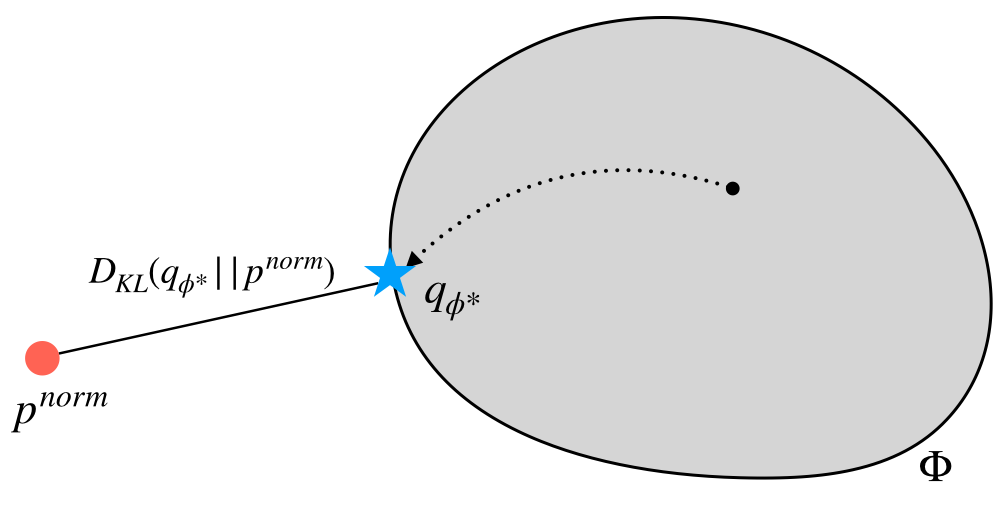
Optimizing \(\phi\) within the variational family (grey area) so that \(q_\phi\) is as close to \(p^{norm}\) as possible.
In the diagram above, we visualize the process of optimizing \(\phi\) to obtain \(q_{\phi^{*}}\) that is closest (in KL-divergence) to \(p^{norm}\), which is the normalized form of \(p\) (i.e. \(p^{norm}(x) = p(x) / \int_{x}{p(x) dx}\)).
Unfortunately, the problem of finding the optimal \(\phi\) is rather difficult in high-dimensional discrete settings (Zhang et al. 2018), which are relevant in many applications (e.g. in tasks such as topic modelling or image segmentation). Let’s see what makes them challenging, and how we can better optimize in discrete settings.
Throwing Darts Blindfolded
As we saw, the problem of maximizing the ELBO is equivalent to finding the \(\phi\) that minimizes the KL divergence from \(q_\phi\) to \(p^{norm}\). This means that we need to figure out where the points of high probability (in \(p^{norm}\)) are, so that we can nudge \(\phi\) to make \(q_\phi\) place high probability on those points.
Finding these points of high probability can be challenging, especially in high dimensions where stochastic/sampling approaches are ineffective (curse of dimensionality), and especially in discrete settings. In discrete settings, we cannot take gradients with respect to samples to get information on where the high probability points are (i.e. the so-called reparameterization trick in continuous settings).
We’ll refer to the sampling-based approach as stochastic optimization.
Stochastic Optimization (sampling)
When using stochastic optimization, we perform gradient ascent using Monte-Carlo estimates of the ELBO gradients. In discrete settings, we rely on the score function estimator to give estimates of the ELBO gradients, by taking samples \(x \sim q_\phi\).
\[\nabla_\phi \mathbb{E}_{x\sim q_\phi} [ \log p(x) - \log q_\phi(x) ] = \mathbb{E}_{x\sim q_\phi} [ (\log p(x) - \log q_\phi(x)) \nabla_\phi \log q_\phi(x) ]\]Unfortunately, the estimates can vary wildly depending on the samples that we get (high variance), especially when \(x\) is high-dimensional.
In essence, stochastic optimization in high-dimensional discrete settings is like throwing darts blindfolded, with your friend telling you only if you hit the bullseye, but not which direction to adjust your throws. Except instead of a circular dartboard, you’re throwing helplessly into an N-dimensional lattice.
If Not Sampling, Then What?
Instead of relying on just a few samples to estimate the ELBO gradient, what if we directly compute the ELBO gradient? This would be equivalent to considering all samples at once! We would see exactly where the points of high probability are, and know exactly how to nudge \(\phi\) to distribute probability mass onto those points. We’ll refer to this direct computation approach as analytic optimization.
Analytic Optimization (direct computation)
When using analytic optimization, we compute the ELBO gradient \(\nabla_\phi \mathbb{E}_{x\sim q_\phi} [ \log p(x) - \log q_\phi(x)]\) directly, without sampling. This gives us exact (zero variance) values of the ELBO gradient, and is equivalent to taking samples everywhere at once! We can then optimize \(\phi\) more easily to get tighter ELBOs.
Unfortunately, analytic computation of the ELBO gradient is rather difficult, and has typically been limited to simple mean-field variational families. In order to compute the expectation without actually taking samples everywhere (which would not be practical in high dimensions), we would need certain “structure” on \(q_\phi\) and \(p\).
The Tradeoff
It appears that we are left with a tradeoff between 1) a simpler variational family where we can optimize \(\phi\) analytically and 2) a more expressive variational family where we resort to stochastic optimization of \(\phi\).
- On one hand, we can choose a simple variational family where we can perform analytic optimization (hence solving the optimization problem is simpler), but the optimal ELBO (i.e. \(\sup_\phi\) ELBO) is low.
- On the other hand, we can choose an expressive variational family where the optimal ELBO is high, but the optimization problem – actually finding the \(\phi\) that maximizes the ELBO – is hard. There may be no efficient methods to compute the ELBO gradients, and we may have to resort to stochastic optimization using high-variance estimates.
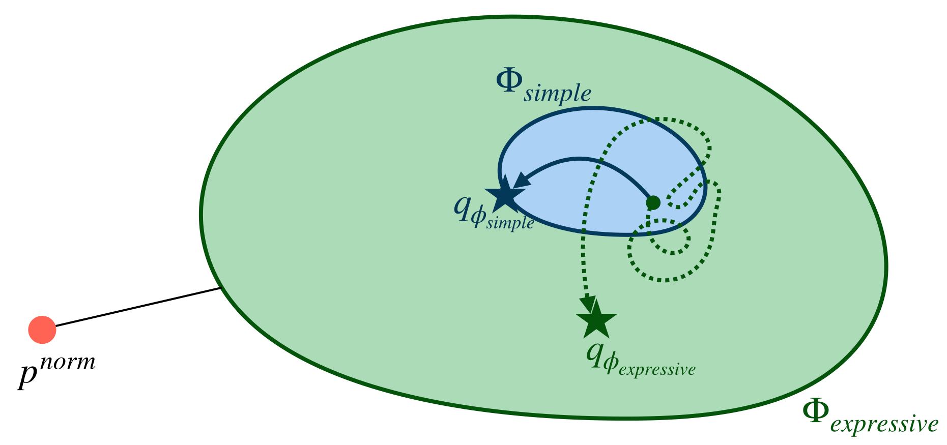
Using a simple family (in blue) makes it easy to optimize, but the optimal solution is not great (far away from \(p^{norm}\)). Using an expressive family (in green) allows us to be close to \(p^{norm}\), but optimization is very difficult/noisy, as shown by the dotted path.
This tradeoff is quite inconvenient. We would like to get the best of both worlds – that is, to have an expressive variational family that allows for analytic/easy optimization of \(\phi\).
Best of Both Worlds
To get a more flexible variational family that still allows for analytic optimization, we look towards tractable probabilistic models that go under the name of Arithmetic Circuits, Sum-Product Networks, and Probabilistic Circuits.
Probabilistic Circuits
Probabilistic Circuits (PCs) is an umbrella term for Arithmetic Circuits (ACs) and Sum-Product Networks (SPNs). These models induce a probability distribution using a circuit with sum and product nodes. Edges in the circuit are parameterized by weights \(\phi\). These models are tractable in the sense that we can compute exact likelihoods and marginals (such as \(p(x_1 \vert x_0)\)) of their probability distributions. For details on how to do this, here is a good resource (Choi, Vergari, and Van den Broeck 2020). Turns out, not only can we compute likelihoods and marginals tractably with these models, but we can also compute certain ELBO gradients analytically when using these models as the variational distribution!
Details of Probabilistic Circuits (Click to expand)
These models gain their tractability from two main properties: decomposability and determinism.
-
Decomposability says that children of a product node have disjoint scopes (depend on disjoint sets of variables).
-
Determinism says that children of a sum node must be mutually exclusive – for any input \(x\) only one child can evaluate to non-zero.
Arithmetic Circuits enforce both properties. Sum-Product Networks were introduced later by dropping the property of determinism. Selective-SPNs refers to SPNs that are deterministic, and are therefore entirely equivalent to Arithmetic Circuits. Here’s a good resource for learning more about how they relate (Choi and Darwiche 2017). (In this work we use the terms ACs, SPNs, and PCs rather interchangeably.)
We show that the properties of decomposability and determinism enable analytic computation of the ELBO (and therefore its gradients by automatic differentiation), if we have the log-density of the target model \(p\) as a polynomial1. Some of these results were introduced in this paper (Lowd and Domingos 2010), but in our work we improved the complexity of computing entropy from quadratic to linear, which was crucial for scaling to bigger problems. Here, we briefly go over the main ideas.
If we think about these models as computation graphs with the root being the output of the model, then we just have to show how to (recursively) compute the ELBO of a parent node from the ELBO of the children nodes. Let \(g_i\) denote a sum or product node in the selective-SPN, and \({g_j : j \in ch(i)}\) denote the children of \(g_i\). We first write the ELBO as a cross-entropy term an an entropy term, and we’ll roughly see how to compute them recursively.
\[\begin{aligned} & \underbrace{ \mathbb{E}_{x \sim g_i} [ \log p(x) ]}_{\text{- cross-entropy}} \underbrace{- \mathbb{E}_{x \sim g_i} [\log g_i(x)]}_{\text{entropy}} \end{aligned}\]If \(g_i\) is a sum node
At sum nodes, \(g_i(x) = \sum_{j \in ch(i)} \alpha_{ij}g_j(x)\), where \(\sum_j{\alpha_{ij}}=1\) and children are mutually exclusive. The cross-entropy term breaks down by linearity of expectations. The entropy term looks like this when expanded out:
\[\mathbb{E}_{x \sim g_i} [\log g_i(x)] = \sum_{j \in ch(i)} \alpha_{ij} \mathbb{E}_{x \sim g_j} [\log \sum_{k \in ch(i)} \alpha_{ik} g_k(x)]\]But since the children are mutually exclusive, this simplifies to the following:
\[\begin{aligned} & \sum_{j \in ch(i)} \alpha_{ij} \mathbb{E}_{x \sim g_j} [\log \alpha_{ij} g_j(x)]\\ = & \sum_{j \in ch(i)} \alpha_{ij} \log \alpha_{ij} + \alpha_{ij} \mathbb{E}_{x \sim g_j} [ \log g_j(x)] \end{aligned}\]which enables easy recursive computation.
If \(g_i\) is a product node
At product nodes, \(g_i(x) = \prod_{j \in ch(i)} g_j(x)\), where children have disjoint scopes2 and are hence independent. The cross-entropy term decomposes because \(\log p(x)\) is a polynomial, so we can split the variables of in the polynomial according to the scopes of the children nodes. The entropy term also breaks down easily due to independence.
\[\begin{aligned} & - \mathbb{E}_{x \sim g_i} [\log g_i(x)] = - \sum_{j \in ch(i)} \mathbb{E}_{x \sim g_j} [\log g_j(x)]\\ \end{aligned}\]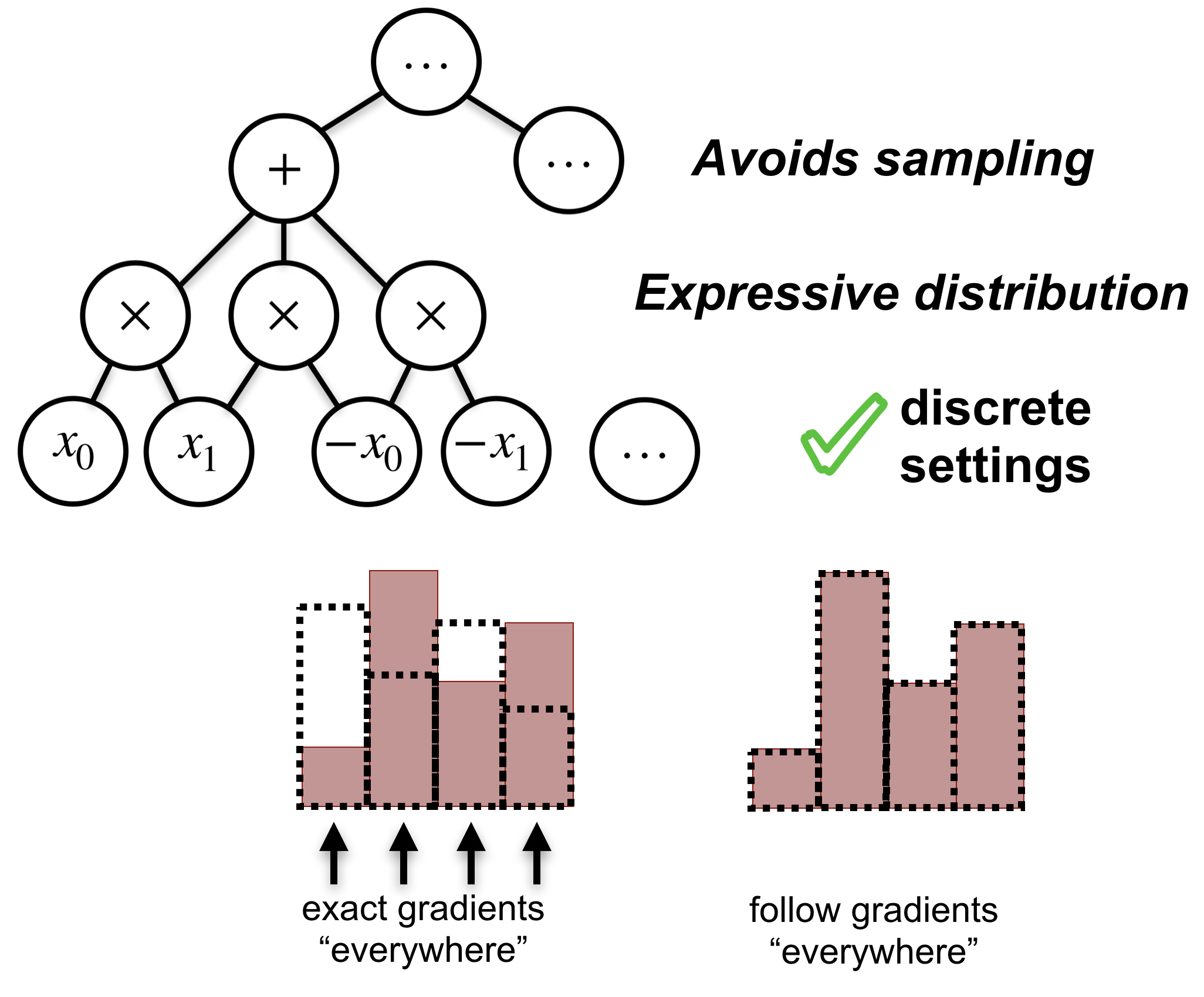
By computing the ELBO gradients analytically (no variance!), we are essentially able to follow the gradients ‘everywhere’ at once, even in high-dimensional discrete settings.
Toy Example (Click to expand)
Consider a toy example over \(3\) binary variables: \(x \in \{-1,1\}^3\). Let’s see how we can use an SPN as the variational family to compute the ELBO analytically.
Suppose the target unnormalized density is \(\log p(x) = 0.5 x_1 x_2\), and the variational distribution \(q_\phi\) is a (selective-)SPN.
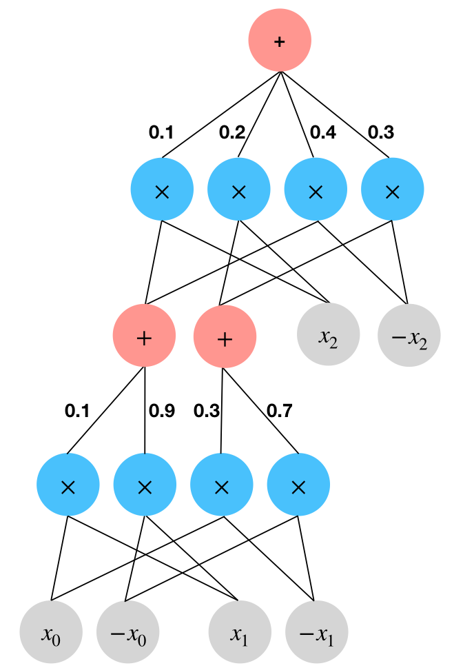
Using an SPN as the variational distribution \(q_\phi\): sum nodes are in red and product nodes are in blue.
To get the probability of an input, we simply set the corresponding leaf nodes to \(1\) and evaluate the weighted sums and the products. So, our SPN encodes the following distribution over the \(2^3=8\) possible inputs:
| \(x = x_0 x_1 x_2\) | \(q_\phi(x)\) |
|---|---|
| \(+1 +1 +1\) | \(0.1 * 0.1 = 0.01\) |
| \(+1 +1 -1\) | \(0.1 * 0.4 = 0.04\) |
| \(+1 -1 +1\) | \(0.3 * 0.2 = 0.09\) |
| \(+1 -1 -1\) | \(0.3 * 0.3 = 0.09\) |
| \(-1 +1 +1\) | \(0.9 * 0.1 = 0.09\) |
| \(-1 +1 -1\) | \(0.9 * 0.4 = 0.36\) |
| \(-1 -1 +1\) | \(0.7 * 0.2 = 0.14\) |
| \(-1 -1 -1\) | \(0.7 * 0.3 = 0.21\) |
To compute the ELBO we’ll first compute the cross-entropy term \(\mathbb{E}_{x \sim q_\phi} [\log p(x)] = - 0.5 \mathbb{E}_{x \sim q_\phi} [ x_1 x_2 ]\). We set the leaves accordingly:
- \(x_1\) and \(x_2\) are set to \(+1\) since they are positive.
- \(- x_1\) and \(- x_2\) are set to \(-1\) since they are negative.
- \(x_0\) and \(-x_0\) are both set to \(1\) since they do not appear in the monomial \(x_1 x_2\).
Then we simply evaluate the circuit, taking weighted sums at sum nodes and product at product nodes. We see in the following diagram that the cross entropy term evaluates to \(-0.5 * -0.2 = 0.1\).
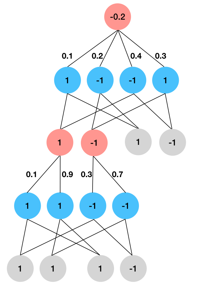
Cross Entropy. Positive leaves are set to \(+1\), negative leaves are set to \(-1\), and leaves that do not appear in the term are set to \(+1\). We evaluate the circuit bottom-up to compute the expectation analytically. For \(\log p\) that is a polynomial, we simply evaluate each monomial separately and add them together at the end.
Finally, we need to compute the entropy term. The exact computation rules are described in the earlier section. In brief, leaves are deterministic so their entropies are set to \(0\). At product nodes we take the sum of entropies of children, and at sum nodes we take a weighted sum of entropies of children plus the entropy of the weights. We see in the following diagram that the entropy term evaluates to \(1.7478\).
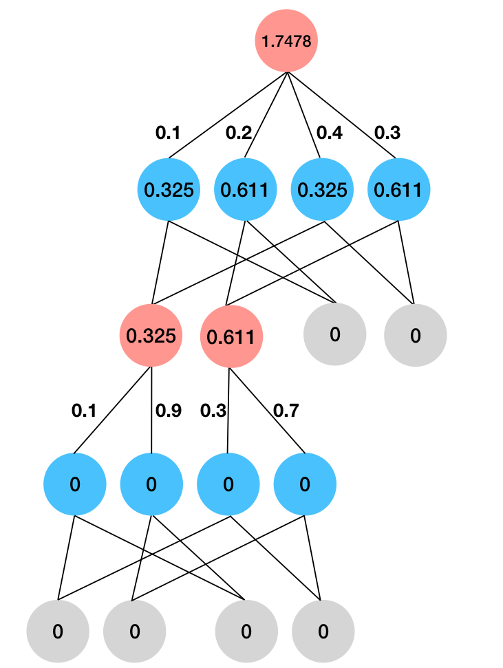
Entropy. Leaves are set to \(0\). At product nodes we add the entropy. At sum nodes we take weight sum of entropies and add the entropy of the weights.
Great! We’ve computed the ELBO without sampling or enumerating all possible inputs! We can simply rely on autodiff to get the exact gradients with respect to \(\phi\), and optimize \(\phi\) easily. The process takes time linear in the size of the SPN, which scales well to high dimensions.
Let’s do a quick sanity check of our result.
\[\mathbb{E}_{x \sim q_\phi} [\log p(x)] - \mathbb{E}_{x \sim q_\phi} [\log q(x)] = 0.1 + 1.7478 = 1.8478\]| \(x = x_0 x_1 x_2\) | \(q_\phi(x)\) | \(p(x)\) | \(q_\phi(x) * (\log p(x) - \log q_\phi(x))\) |
|---|---|---|---|
| \(+1 +1 +1\) | \(0.01\) | \(e^{-0.5}\) | \(0.0411\) |
| \(+1 +1 -1\) | \(0.04\) | \(e^{0.5}\) | \(0.1488\) |
| \(+1 -1 +1\) | \(0.06\) | \(e^{0.5}\) | \(0.1988\) |
| \(+1 -1 -1\) | \(0.09\) | \(e^{-0.5}\) | \(0.1717\) |
| \(-1 +1 +1\) | \(0.09\) | \(e^{-0.5}\) | \(0.1717\) |
| \(-1 +1 -1\) | \(0.36\) | \(e^{0.5}\) | \(0.5478\) |
| \(-1 -1 +1\) | \(0.14\) | \(e^{0.5}\) | \(0.3452\) |
| \(-1 -1 -1\) | \(0.21\) | \(e^{-0.5}\) | \(0.2227\) |
| total | \(1.00\) | \(e^{2.1996}\) | \(1.8478\) |
Indeed the ELBO is \(1.8478\), which lower bounds the true log partition function \(\log Z = 2.1996\). We can even check that the gap of \(2.1996 - 1.8478 = 0.3518\) indeed matches the value \(KL(q_\phi \vert \vert p^{norm})\).
We showed that we can compute the ELBO analytically when using selective-SPNs as the variational distribution \(q_\phi\). Then, we simply use automatic differentiation to get the exact gradients of the ELBO with respect to the parameters \(\phi\) of the SPN, and gradient ascent to optimize the SPN. Some analysis will show that each optimization step takes time \(O(tm)\) where \(t\) is the number of factors when expressing the target distribution \(p\) in log-linear form, and \(m\) is the size of our variational distribution \(q\) (# of edges in the SPN). With GPU-optimization, we were able to scale to target models with more than 1,000 factors/variables and SPNs with more than 100,000 edges.
Using SPNs, we computed better estimates of the partition function compared to standard methods such as mean-field variational inference (MF-VI) or Loopy Belief Propagation. Compared to MF-VI, we were able to get ELBOs that are 4 times tighter on 16x16 Ising models. We also experimented on factor graphs used for topic modelling and image segmentation, where our method gave the best ELBO on 22 out of 23 factor graphs.
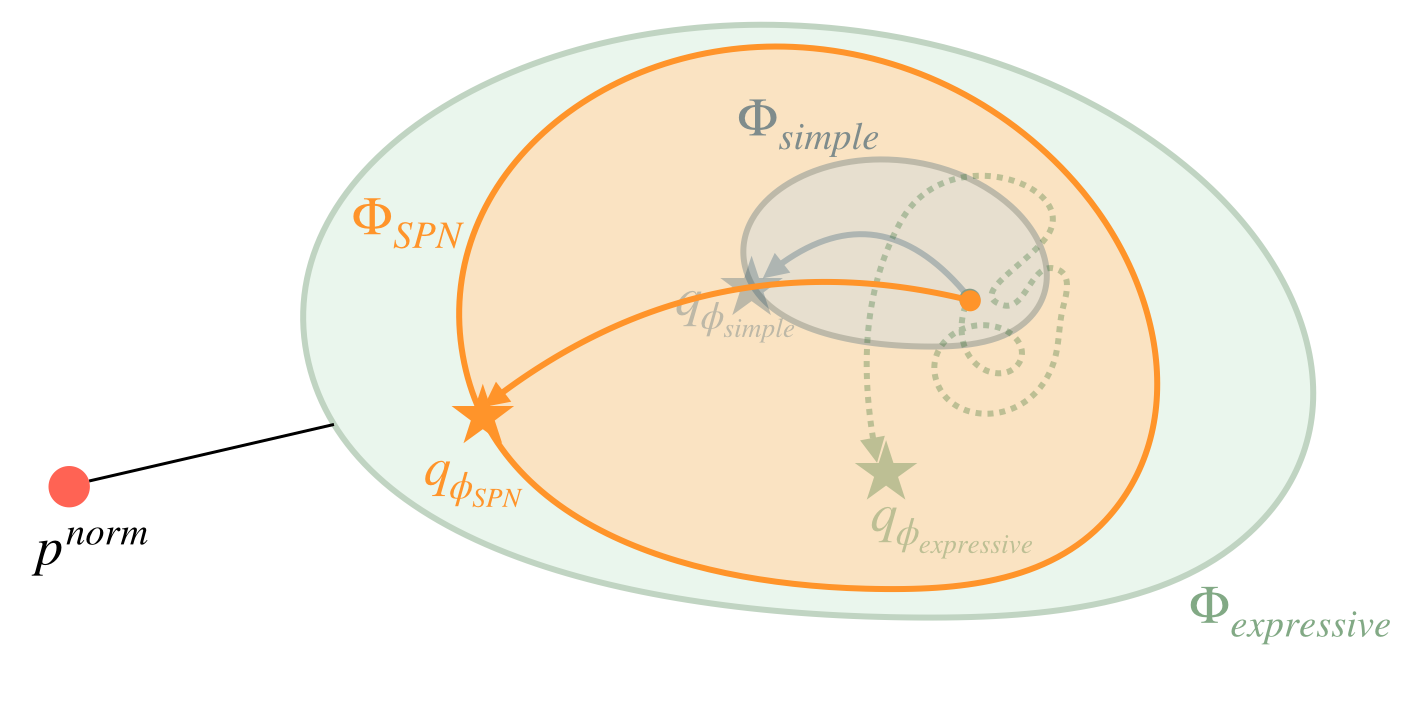
Using SPNs (in orange), we get more expressive power while still allowing easy/analytic optimization. The combination of expressivity and tractability gives us better ELBOs, and make SPNs suitable as the variational family for high-dimensional discrete settings.
Summary
Variational inference in high-dimensional discrete settings is challenging since sampling for the ELBO gradient works poorly and directly computing the ELBO gradient is difficult. To address this problem we proposed to use SPNs as the variational family – the combination of expressivity and the support of analytic optimization makes them suitable for high-dimensional discrete settings. To use these tractable probabilistic models in your own project, feel free to check out our code in Python, or check out this package in Julia from folks at UCLA.
Footnotes
-
This might seem somewhat limiting, but every real-valued binary function (\(\log p\) in this case) can be written as a polynomial via Discrete Fourier Transform. ↩
-
For example, a product node \(g_i\) may define a probability distribution over the variable set (a.k.a. scope) \(\{0,1,2,3\}\), with two children nodes \(g_{j1}\) and \(g_{j2}\) that define probability distributions over variable sets \(\{0,1\}\) and \(\{2,3\}\), respectively. When we write \(g_{j1}(x)\), for example, we are implicitly dropping out all the variables outside the scope of the node \(g_{j1}\). ↩
References
- Zhang, Cheng, Judith Bütepage, Hedvig Kjellström, and Stephan Mandt. 2018. “Advances in Variational Inference.” IEEE Transactions on Pattern Analysis and Machine Intelligence 41 (8): 2008–26.
- Choi, YooJung, Antonio Vergari, and Guy Van den Broeck. 2020. “Probabilistic Circuits: A Unifying Framework for Tractable Probabilistic Models,” October. http://starai.cs.ucla.edu/papers/ProbCirc20.pdf.
- Choi, Arthur, and Adnan Darwiche. 2017. “On Relaxing Determinism in Arithmetic Circuits.” In ICML.
- Lowd, Daniel, and Pedro Domingos. 2010. “Approximate Inference by Compilation to Arithmetic Circuits.” Advances in Neural Information Processing Systems 23: 1477–85.