Variational Rejection Sampling
TL;DR: Variational learning of intractable posteriors is computationally efficient, but the resulting approximations can be poor. We propose a general approach to increase the flexibility of any variational family by augmenting a parameterized variational posterior with a differentiable and tunable accept-reject step. The rejection rate for the resulting resampled posterior can be adaptively controlled to monotonically trade-off computation for statistical accuracy, with the resampled posterior matching the true posterior in the limit.
The key computational challenge in high-dimensional Bayesian statistics is to approximate intractable posterior densities. Consider the standard Bayesian inference setting where we have a set of latent variables \(\mathbf{z}\) that explain the observed data \(\mathbf{x}\). We can perform posterior inference for such a model by following a simple recipe. First, we specify some apriori beliefs about \(\mathbf{z}\) through a prior density \(p(\mathbf{z})\). Next, we observe a data point \(\mathbf{x}\) which relates to the latent variables through the likelihood \(p(\mathbf{x} \vert \mathbf{z})\). Finally, we can update our apriori beliefs regarding \(\mathbf{z}\) through the posterior density \(p(\mathbf{z} \vert \mathbf{x})\). Using Bayes Rule, we have:
\[p(\mathbf{z} \vert \mathbf{x}) = \frac{p(\mathbf{x}, \mathbf{z})}{p(\mathbf{x})} = \frac{p(\mathbf{x} \vert \mathbf{z}) p(\mathbf{z})}{\int_\mathbf{z} p(\mathbf{x}, \mathbf{z}) \mathrm{d} \mathbf{z}}\]For a high-dimensional latent space, the task of evaluating the posterior is intractable as it involves integrating over all the possible latent factors to compute the marginal density \(p(\mathbf{x})\). This necessitates the use of approximation inference techniques. There are broadly two classes of approximate inference techniques: variational inference and Monte Carlo methods.
Variational Inference
Variational inference is an approximation technique that casts posterior inference as an optimization problem. In variational inference, we consider a parametric family of densities and pick the member of this family that minimizes the KL divergence with the true posterior.
Application: Latent Variable Modeling using Variational Bayes
Suppose we observe a finite dataset of samples \(D = \{\mathbf{x}_1, \mathbf{x}_2, \ldots, \mathbf{x}_n\}\) sampled from an unknown data distribution and our goal is to approximate the data distribution as closely as possible. A standard approach is to learn a parameterized latent variable generative model that maximizes the marginal log-likelihood averaged over the entire dataset. That is, we consider the following optimization problem:
\[\max_{\theta} \frac{1}{n} \sum_{i} \log p_\theta(\mathbf{x}_i).\]Evaluating and optimizing the marginal log-likelihood \(\log p_\theta(\mathbf{x})\) for any arbitrary data point \(\mathbf{x}\) is computationally intractable. We can sidestep this difficulty by introducing an amortized variational posterior \(q_\phi(\mathbf{z} \vert \mathbf{x})\) with parameters \(\phi\).
\[\log p_\theta(\mathbf{x}) = \mathbb{E}_{q_\phi} \left[ \log p_\theta(\mathbf{x}, \mathbf{z}) \right] - \mathbb{E}_{q_\phi} \left[ \log q_\phi(\mathbf{z} \vert \mathbf{x}) \right] + KL(q(\mathbf{z} \vert \mathbf{x}) \Vert p(\mathbf{z} \vert \mathbf{x})) \\ \geq \mathbb{E}_{q_\phi} \left[ \log p_\theta(\mathbf{x}, \mathbf{z}) \right] - \mathbb{E}_{q_\phi} \left[ \log q_\phi(\mathbf{z} \vert \mathbf{x}) \right]\]The evidence lower bound (ELBO) objective above is tight when the variational posterior matches the true posterior, i.e., \(q_\phi(\mathbf{z} \vert \mathbf{x}) = p_\theta(\mathbf{z} \vert \mathbf{x})\).
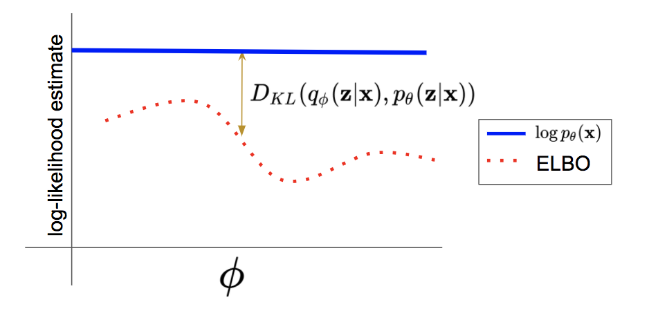
The above illustration highlights the difficulty with variational learning. For simplicity we fix \(\theta\) and pick an arbitrary variational family of posterior distributions. For any choice of variational parameters \(\phi\) within this family, we get a lower bound to the marginal log-likelihood. However, if the variational family is not expressive enough to represent the true posterior, then there will always be a gap between the marginal log-likelihood and the ELBO, which is given by the KL divergence between the variational posterior and the true posterior.
Rejection Sampling
Many scenarios for Bayesian inference only require expectations with respect to a posterior distribution. For such tasks, we can perform implicit posterior inference using Monte Carlo methods. These methods simulate samples from the target posterior distribution, which can then be used for estimating expectations.
In this post, we turn our attention to one of the simplest Monte Carlo methods, called rejection sampling. The geometric intuition for rejection sampling is best illustrated using a textbook example.
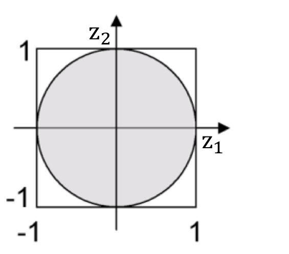
Let us assume we want to sample a point uniformly from the unit circle shown above. In order to do so, we first characterize an easy-to-sample envelope density that completely covers the desired circle, such as the square with side length \(2\) centered at the origin. Sampling from a uniform distribution over the square is easy; we can independently sample the \(z_1\) and \(z_2\) coordinates between \(-1\) and \(1\). If the sample generated falls within the circle, then we accept the sample. Else, we reject it (we discard it) and repeat the process until a sample is accepted. It is easy to see this procedure is correct.
More generally in order to draw samples from a target density \(t(\mathbf{z})\), a rejection sampler first draws samples from an easy-to-sample source density \(\mathbf{z} \sim s(\mathbf{z})\) with a larger-or-equal support, i.e., \(s(\mathbf{z}) > 0\) wherever \(t(\mathbf{z}) > 0\). Then, provided we have a fixed, finite upper bound \(M \in [1,\infty)\) on the likelihood ratio \(\frac{t(\mathbf{z})}{s(\mathbf{z})}\) that holds for all \(\mathbf{z}\), we can obtain samples from the target by accepting samples from \(s(\mathbf{z})\) with a probability \(a_{s,t,M}(\mathbf{z}) = \frac{t(\mathbf{z})}{M s(\mathbf{z})}\). Note that the acceptance probability is guaranteed to be less than or equal to \(1\) since \(M\) defines an upper bound. The overall probability of any accepted sample \(\mathbf{z}\) is proportional to \(\tfrac{t(\mathbf{z})}{M s(\mathbf{z})} \times s(\mathbf{z})\).
For rejection sampling to work in practice, we need two desiderata. First, the source density should be close to the the target density. Second, the constant \(M\) has to be large enough such that it is a valid upper bound for the likelihood ratio and the acceptance probability does not exceed \(1\). In principle, any upper bound on the likelihood ratio that holds for all \(\mathbf{z}\) suffices to ensure the correctness for rejection sampling. However, even for a fixed source and target density, the optimal value \(M^\ast\) is the one that attains the tightest upper bound. If we let \(M>M^\ast\), then the sampling procedure is still valid but becomes computationally inefficient due to a higher rejection rate.
For instance, consider the case where the target density is discrete and non-zero for only four states as shown below.
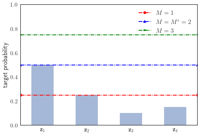
For rejection sampling, let us assume we choose the source density to be uniform over the four points. The acceptance probability for any point \(\mathbf{z}\) sampled from the source density is given by:
\[a_{s,t,M}(\mathbf{z}) =\begin{cases} \frac{0.50}{M\times 0.25}\text{ if }\mathbf{z}=\mathbf{z}^{(1)}, \\ \frac{0.25}{M\times 0.25}\text{ if }\mathbf{z}=\mathbf{z}^{(2)}, \\ \frac{0.10}{M\times 0.25}\text{ if }\mathbf{z}=\mathbf{z}^{(3)}, \\ \frac{0.15}{M\times 0.25}\text{ if }\mathbf{z}=\mathbf{z}^{(4)}. \end{cases}\]Depending on the choice of \(M\), there are three possible scenarios:
- \(M = M^\ast = 2\) (blue): This is the tightest possible upper bound giving an exact rejection sampler with the best computational efficiency with all states sampled as per their true, target probabilities.
- \(M > 2\) (green): This defines an exact rejection sampler, but has a high rejection rate and hence, poor computational efficiency.
- \(M < 2\) (red): This defines an inexact rejection sampler, since certain states are oversampled. For instance, if \(M=1\), then \(\mathbf{z}^{(1)}\) and \(\mathbf{z}^{(2)}\) are sampled with the same probability which is incorrect as per the target probabilities.
Hence, the choice of \(M\) has a significant impact on the correctness and computational efficiency of rejection sampling. Finally, note that if the source matches the target then the tightest upper bound is trivially given by \(M = M^\ast = 1\).
Comparison summary
Both variational inference and rejection sampling (along with other Monte Carlo methods) are widely used techniques in machine learning for approximate inference. While variational inference is efficient and is able to directly leverage advancements in optimization, the model performance depends critically on the quality of variational approximation. Particularly when the data is high-dimensional, it is unlikely that relatively simple approximations such as mean-field, inspite of expressive parameterization based on neural networks, can capture the full complexity of the true posterior distribution. Rejection sampling on the other hand is exact, but a poor choice of the source distribution and/or the upper bound on the likelihood ratio can lead to a high rejection rate, i.e., a very computationally inefficient procedure.
We now discuss the variational rejection sampling (VRS) framework with a goal of attaining the best of both worlds. In particular, it seeks to improve the statistical accuracy of variational approximations in latent variable generative models using rejection sampling while still controlling for computational efficiency.
Variational Rejection Sampling
In VRS, we consider an implicit variational posterior defined through the following two-step variational rejection sampler:
- Step 1: Draw a sample \(\mathbf{z} \sim q_\phi (\mathbf{z} \vert \mathbf{x})\) for any vanilla variational posterior \(q_\phi (\mathbf{z} \vert \mathbf{x})\).
- Step 2: Draw a uniform number \(u \in \mathrm{Unif}[0,1]\). If \(u \leq a_{\theta, \phi}(\mathbf{z} \vert \mathbf{x}, T)\), accept \(\mathbf{z}\) else reject \(\mathbf{z}\) and repeat Step 1.
where \(a_{\theta, \phi}(\mathbf{z} \vert \mathbf{x}, T) \in (0, 1]\) is an acceptance probability function that depends on \(\theta, \phi\), and an additional threshold parameter \(T\). Note that \(a_{\theta, \phi}(\mathbf{z} \vert \mathbf{x}, T)\) is not a density over \(\mathbf{z}\), but denotes the parameter for a Bernoulli random variable that signifies the probability with which \(\mathbf{z}\) should be accepted.
The implicit variational posterior is referred to henceforth as a resampled posterior distribution and its density can be formally expressed as:
\[r_{\theta, \phi}(\mathbf{z} \vert \mathbf{x}, T) \propto q_\phi (\mathbf{z} \vert \mathbf{x}) a_{\theta, \phi}(\mathbf{z} \vert \mathbf{x}, T).\]The resampled posterior represents a distribution over all the possible outputs (i.e. accepted samples) of the rejection sampler defined previously. The normalization constant for the resampled posterior, \(Z_R(\mathbf{x}, T) = \mathbb{E}_{Q}[a_{\theta, \phi}(\mathbf{z} \vert \mathbf{x}, T)]\) gives the average probability of acceptance for any sample from \(q_\phi (\mathbf{z} \vert \mathbf{x})\) and governs the average runtime for obtaining a single sample from \(r_{\theta, \phi}(\mathbf{z} \vert \mathbf{x}, T)\). This constant is generally computationally intractable as it involves an expectation with respect to a high-dimensional distribution, but is however unnecessary for defining the variational rejection sampler.
Further, we can state the ELBO for the VRS learning objective, which simply substitutes the variational posterior with the resampled posterior:
\[\max_{\theta, \phi} \mathbb{E}_{r_{\theta, \phi}(\mathbf{z} \vert \mathbf{x}, T)} \left[ \log p_\theta(\mathbf{x}, \mathbf{z}) \right] - \mathbb{E}_{r_{\theta, \phi}(\mathbf{z} \vert \mathbf{x}, T)} \left[ \log r_{\theta, \phi}(\mathbf{z} \vert \mathbf{x}, T) \right]\]We now discuss the specification of the acceptance probability function and gradient estimators for efficient optimization of the above objective.
Monotonically trading computation for statistical accuracy
Recall that in vanilla rejection sampling, the acceptance probability for any sample can be specified under the following two assumptions:
- The source \(s(\mathbf{z})\) and target \(t(\mathbf{z})\) densities can be evaluated at any given point.
- An upper bound on the likelihood ratio of the target and the source (i.e., \(\frac{t(\mathbf{z})}{s(\mathbf{z})}\)) is known.
For learning a latent variable generative model through ELBO maximization, the source corresponds to the variational posterior \(q_\phi (\mathbf{z} \vert \mathbf{x})\) and the target is given by the true posterior \(p_\theta(\mathbf{z} \vert \mathbf{x})\). Assuming the supports of the source and target match, this gives us the following acceptance probability function:
\[a_{\theta, \phi}(\mathbf{z}\vert \mathbf{x}, M) = \frac{p_\theta(\mathbf{z} \vert \mathbf{x} )}{Mq_\phi (\mathbf{z} \vert \mathbf{x})}\]where \(M\) is an upper bound on the likelihood ratio \(\frac{p_\theta(\mathbf{z} \vert \mathbf{x})}{q_\phi (\mathbf{z} \vert \mathbf{x})}\). However, the true posterior is only known up to a normalization constant \(p_\theta(\mathbf{x})\) via \(p_\theta(\mathbf{x}, \mathbf{z})\). We can use then rewrite the acceptance probability function:
\[a_{\theta, \phi}(\mathbf{z}\vert \mathbf{x}, M') = \frac{p_\theta(\mathbf{x}, \mathbf{z})}{M p_\theta(\mathbf{x})q_\phi (\mathbf{z} \vert \mathbf{x})} = \frac{p_\theta(\mathbf{x}, \mathbf{z})}{M'q_\phi (\mathbf{z} \vert \mathbf{x})}\]for some quantity \(M' = M p_\theta(\mathbf{x})\) that is a constant for a fixed \(\theta\) and \(\mathbf{x}\). Consequently, \(M'\) is required to be an upper bound for the ratio \(\frac{p_\theta(\mathbf{x}, \mathbf{z})}{q_\phi (\mathbf{z} \vert \mathbf{x})}\).
We are faced with yet another challenge. In practice, we do not know how large \(M'\) should be, and using a loose bound (an excessively large value) leads to an increase in computation due to a higher rejection rate. We transform this challenge into an opportunity, and instead consider a variant of rejection sampling, where in we allow the user to specify a threshold \(M'\) based on the available computation. The threshold is translated into a value \(M'\) that is no longer guaranteed to dominate the likelihood ratio across the entire state space. Since we cannot allow the acceptance probability to exceed \(1\), we set the acceptance probability for VRS to be minimum of \(1\) and the acceptance probability for a vanilla rejection sampler:
\[a_{\theta, \phi}(\mathbf{z}\vert \mathbf{x}, M') = \min\left[1, \frac{p_\theta(\mathbf{x}, \mathbf{z})}{M'q_\phi (\mathbf{z} \vert \mathbf{x})}\right]\]for some user-specified threshold \(M'\). Finally, we relax the \(\min\) operator to consider a differentiable approximation and let \(M'=e^{-T}\) to obtain the following acceptance probability function (derivation in the paper):
\[\log a_{\theta, \phi}(\mathbf{z}\vert \mathbf{x}, T) = - \log [1+ \exp(l_{\theta, \phi}(\mathbf{z} \vert \mathbf{x}, T))]\]where \(l_{\theta, \phi}(\mathbf{z} \vert \mathbf{x}, T) = - \log p_\theta(\mathbf{x}, \mathbf{z}) + \log q_\phi(\mathbf{z} \vert \mathbf{x}) - T\). Hence, the negative log-acceptance probability is a softplus over \(l_{\theta, \phi}(\mathbf{z} \vert \mathbf{x}, T)\).
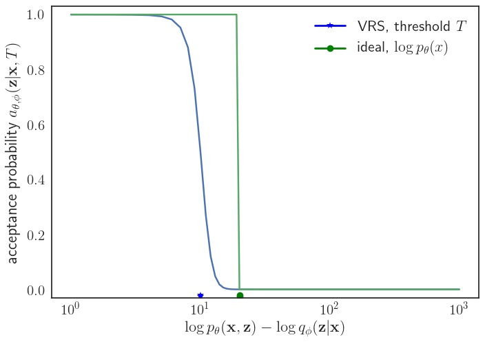
VRS acceptance probability for samples from the variational posterior that disagree with the unnormalized true posterior beyond a threshold margin (blue star) decays exponentially. For a perfect variational posterior, the acceptance probability for a rejection sampler with the tightest upper bound is a step function at \(\log p_\theta(\mathbf{x})\) (green circle).
The choice of acceptance probability function above enforces the following behavior for the samples generated by the resampled posterior: samples from the approximate posterior that disagree with the target posterior (as measured by the difference in log-likelihoods \(\log p_\theta(\mathbf{x}, \mathbf{z}) - \log q_\phi(\mathbf{z} \vert \mathbf{x})\)) beyond a level implied by the corresponding threshold \(T\) have an exponentially decaying probability of getting accepted, while leaving the remaining samples with negligible interference from resampling.
To get some intuition for the VRS acceptance probability function, note that in the ideal setting when \(q_\phi(\mathbf{z} \vert \mathbf{x})\) matches the true posterior, \(p_\theta(\mathbf{z} \vert \mathbf{x})\), the tightest upper bound given by \(M=1\) and hence, \(M'=p_\theta(\mathbf{x})\). The acceptance probability function for vanilla rejection sampling in this case is simply a step function at \(\log p_\theta(\mathbf{x})\). Hence, the VRS acceptance probability function is a shifted, differentiable approximation of the idealized acceptance probability. Importantly, we can show a stronger key result for the VRS acceptance probability function:
For fixed \(\theta, \phi\), the KL divergence between the approximate and true posteriors, \(\mathtt{KL}(r_{\theta, \phi}(\mathbf{z} \vert \mathbf{x}, T) \Vert p_\theta(\mathbf{z} \vert \mathbf{x}))\) is monotonically increasing in \(T\).
Hence, the threshold \(T\) acts as a knob for the resampled posterior distribution to trade-off computation for statistical accuracy, alternating between the following extremes:
- As \(T \rightarrow +\infty\), \(r_{\theta, \phi}(\mathbf{z}\vert\mathbf{x}, T)\) is equivalent to \(q_\phi(\mathbf{z}\vert\mathbf{x})\), with perfect sampling efficiency for the accept-reject step i.e., \(a_{\theta, \phi}(\mathbf{z}\vert\mathbf{x}, T)\rightarrow 1 ~\forall\mathbf{z}\).
- As \(T \rightarrow -\infty\), \(r_{\theta, \phi}(\mathbf{z}\vert\mathbf{x}, T)\) is equivalent to \(p_\theta(\mathbf{z}\vert\mathbf{x})\), with the sampling efficiency of a plain rejection sampler with a highly overestimated \(M>>>M^\ast\) i.e., \(a_{\theta, \phi}(\mathbf{z}\vert\mathbf{x}, T)\rightarrow 0 ~\forall\mathbf{z}\).
We illustrate this phenomena on an example 2D discrete target distribution on a \(5 \times 5\) grid, with a uniform variational posterior approximation augmented with threshold-based resampling.
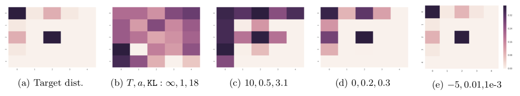
The resampled posterior (b-e) gets closer (in terms of KL divergence) to a target 2D discrete distribution (a) as we decrease the parameter \(T\), which controls the acceptance probability \(a\).
With no resampling (\(T=\infty\)), the approximation is far from the target. As \(T\) is reduced, we observe a progressive improvement in the posterior quality both visually as well as via an estimate of the \(\mathtt{KL}\) divergence from approximation to the target along with an increasing computation cost reflected in the lower acceptance probabilities.
Gradient estimation with unnormalized posteriors
Unlike the standard variational posterior \(q_\phi(\mathbf{z} \vert \mathbf{x})\), the resampled posterior \(r_{\theta, \phi}(\mathbf{z} \vert \mathbf{x}, T)\) is not accessible as a normalized distribution. In fact, the normalization constant (or the partition function) is typically computationally intractable which makes the evaluation of the ELBO objective in the VRS framework challenging. Surprisingly, one of the attractive properties of the VRS framework is that we can sidestep the evaluation of the normalization constant for gradient-based optimization. We skip the derived expressions of the gradients here for brevity; the interested reader can refer to Theorem 2 in the paper.
Crucially, the expressions only involve sampling from the resampled posterior, which as illustrated previously can be done efficiently. In fact, we derive a more general version of the above result that provides an efficient gradient estimator for optimization of ELBO objectives for any unnormalized proposal distribution that can be sampled efficiently, even though evaluation may be computationally intractable due to the partition function.
Overview of algorithmic design and experiments
Training a latent variable generative model using the VRS framework developed is straightforward using stochastic optimization techniques: for every mini-batch of points, we evaluate Monte Carlo gradients for the ELBO objective corresponding to the resampled posterior. The key design question is how do we set the thresholds \(T\)? Ideally, \(T\) should be set in a data-dependent way since the quality of the non-resampled posterior \(q_\phi(\mathbf{z} \vert \mathbf{x})\) can vary signifcantly across different \(\mathbf{x}\). In such a scenario, learning \(T\) in a parametric way is one possibility and interesting direction for future work.
For the current work however, we specify thresholds in a simple quantile-based approach that accepts roughly the top \(\gamma\)-quantile of samples for the random variables \(-\log p_\theta(\mathbf{x}, \mathbf{z}) + \log q_\phi(\mathbf{z} \vert \mathbf{x})\). Since the distribution of the random variables changes during the course of learning, the thresholds are also periodically updated after several epochs of training. Hence, the user needs to specify only a single hyperparameter, \(\gamma\), for specifying the permissible computation. The full algorithm is given in the paper.
We use this algorithm to perform density estimation on the binarized MNIST dataset using sigmoid belief networks with discrete latent variables. These models are particularly hard to optimize since the reparameterization trick is not applicable, leading to gradient estimates with high variance. We show the summary results with VRS models trained compared against the closest baselines on benchmark architectures:
- Single-sample baseline: REBAR (Tucker et al. 2017) continuously relaxes the discrete variational posterior and uses baselines for further variance reduction and using control variates for variance reduction.
| Model | Test NLL (in nats) |
|---|---|
| REBAR | 99.00 |
| VRS (\(\gamma = 0.95\)) | 96.38 |
| VRS (\(\gamma = 0.90\)) | 96.26 |
- Multi-sample baseline: VIMCO (Mnih and Rezende 2016) combines ideas from importance sampling into variational Bayes by sampling \(k\) times from the variational posterior for estimating gradients and using control variates for variance reduction.
| Model | Test NLL (in nats) |
|---|---|
| VIMCO (\(k=2\)) | 93.5 |
| VIMCO (\(k=5\)) | 92.8 |
| VIMCO (\(k=10\)) | 92.6 |
| VIMCO (\(k=50\)) | 91.9 |
| VRS (\(\gamma = 0.95\)) | 91.93 |
| VRS (\(\gamma = 0.90\)) | 91.69 |
Notably, we find empirically the effective number of samples from the posterior for VRS with \(\gamma = 0.90\) is computationally comparable to \(k \approx 20\) which is much lesser than the best performing VIMCO model (\(k=50\)) illustrating the computational efficiency of our approach.
Discussion
The variational rejection sampling is another step in a growing body of work for improving variational posteriors parameterized by deep neural networks with Monte Carlo methods. The specific choice of Monte Carlo technique for such hybrid methods can have a significant effect on the learning: prior work has explored MCMC (Salimans, Kingma, and Welling 2015), importance sampling (Burda, Grosse, and Salakhutdinov 2015), (Mnih and Rezende 2016), and sequential Monte Carlo (Naesseth et al. 2017), (Maddison et al. 2017), (Le et al. 2017). Our work proposes a framework inspired by rejection sampling. While rejection sampling is hardly an attractive Monte Carlo technique in itself, our theoretical and empirical analysis suggests that it can indeed have advantages over other hybrid methods for variational inference and learning.
It is worth noting that many of these Monte Carlo techniques are complimentary and could benefit from each other; for instance, an importance-weighted extension of VRS would assign importance weights to multiple samples drawn from the resampled posterior. Finally, we believe our gradient estimators could be exploited more broadly for stochastic optimization involving Monte-Carlo expectations with respect to other unnormalized distributions, such as energy-based models. If you are interested in reading more about this research, check out the paper below:
Variational Rejection Sampling
Aditya Grover\(^\ast\), Ramki Gummadi\(^\ast\), Miguel L'azaro-Gredilla, Dale Schuurmans, Stefano Ermon
International Conference on Artificial Intelligence and Statistics, 2018.
paper
References
- Tucker, George, Andriy Mnih, Chris J Maddison, John Lawson, and Jascha Sohl-Dickstein. 2017. “REBAR: Low-Variance, Unbiased Gradient Estimates for Discrete Latent Variable Models.” In Advances in Neural Information Processing Systems, 2624–33.
- Mnih, Andriy, and Danilo J Rezende. 2016. “Variational Inference for Monte Carlo Objectives.” In International Conference on Machine Learning.
- Salimans, Tim, Diederik Kingma, and Max Welling. 2015. “Markov Chain Monte Carlo and Variational Inference: Bridging the Gap.” In International Conference on Machine Learning, 1218–26.
- Burda, Yuri, Roger Grosse, and Ruslan Salakhutdinov. 2015. “Importance Weighted Autoencoders.” ArXiv Preprint ArXiv:1509.00519.
- Naesseth, Christian A, Scott W Linderman, Rajesh Ranganath, and David M Blei. 2017. “Variational Sequential Monte Carlo.” ArXiv Preprint ArXiv:1705.11140.
- Maddison, Chris J, John Lawson, George Tucker, Nicolas Heess, Mohammad Norouzi, Andriy Mnih, Arnaud Doucet, and Yee Teh. 2017. “Filtering Variational Objectives.” In Advances in Neural Information Processing Systems, 6576–86.
- Le, Tuan Anh, Maximilian Igl, Tom Jin, Tom Rainforth, and Frank Wood. 2017. “Auto-Encoding Sequential Monte Carlo.” ArXiv Preprint ArXiv:1705.10306.