Sampling methods

In practice, the probabilistic models that we use are often quite complex, and simple algorithms like variable elimination may be too slow for them. In fact, many interesting classes of models may not admit exact polynomial-time solutions at all, and for this reason, much research effort in machine learning is spent on developing algorithms that yield approximate solutions to the inference problem. This section begins our study of such algorithms.

There exist two main families of approximate algorithms: variational methodsVariational inference methods take their name from the calculus of variations, which deals with optimizing functions that take other functions as arguments., which formulate inference as an optimization problem, as well as sampling methods, which produce answers by repeatedly generating random numbers from a distribution of interest.

Sampling methods can be used to perform both marginal and MAP inference queries; in addition, they can compute various interesting quantities, such as expectations \(\E[f(X)]\) of random variables distributed according to a given probabilistic model. Sampling methods have historically been the main way of performing approximate inference, although over the past 15 years variational methods have emerged as viable (and often superior) alternatives.

Sampling from a probability distribution

As a warm-up, let’s think for a minute how we might sample from a multinomial distribution with \(k\) possible outcomes and associated probabilities \(\theta_1, \dotsc, \theta_k\).

Sampling, in general, is not an easy problem. Our computers can only generate samples from very simple distributionsEven those samples are not truly random. They are actually taken from a deterministic sequence whose statistical properties (e.g., running averages) are indistinguishable from a truly random one. We call such sequences pseudorandom., such as the uniform distribution over \([0,1]\). All sampling techniques involve calling some kind of simple subroutine multiple times in a clever way.

In our case, we may reduce sampling from a multinomial variable to sampling a single uniform variable by subdividing a unit interval into \(k\) regions with region \(i\) having size \(\theta_i\). We then sample uniformly from \([0,1]\) and return the value of the region in which our sample falls.

Forward Sampling

⊕
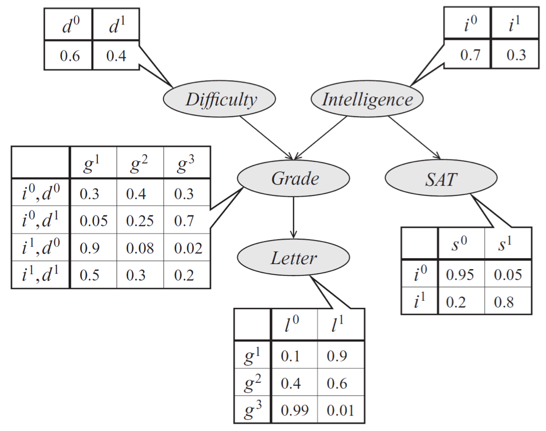
Bayes net model describing the performance of a student on an exam. The distribution can be represented a product of conditional probability distributions specified by tables.

Our technique for sampling from multinomials naturally extends to Bayesian networks with multinomial variables, via a method called ancestral (or forward) sampling. Given a probability \(p(x_1, \dotsc, x_n)\) specified by a Bayes net, we sample variables in topological order. We start by sampling the variables with no parents; then we sample from the next generation by conditioning these variables’ CPDs to values sampled at the first step. We proceed like this until all \(n\) variables have been sampled. Importantly, in a Bayesian network over \(n\) variables, forward sampling allows us to sample from the joint distribution \(\bfx \sim p(\bfx)\) in linear \(O(n)\) time by taking exactly 1 multinomial sample from each CPD.

In our earlier model of a student’s grade, we would first sample an exam difficulty \(d'\) and an intelligence level \(i'\). Then, once we have samples \(d'\) and \(i'\), we generate a student grade \(g'\) from \(p(g \mid d', i')\). At each step, we simply perform standard multinomial sampling.

A former CS228 student has created an interactive web simulation for visualizing Bayesian network forward sampling methods. Feel free to play around with it and, if you do, please submit any feedback or bugs through the Feedback button on the web app.

“Forward sampling” can also be performed efficiently on undirected models if the model can be represented by a clique tree with a small number of variables per node. Calibrate the clique tree, which gives us the marginal distribution over each node, and choose a node to be the root. Then, marginalize over variables in the root node to get the marginal for a single variable. Once the marginal for a single variable \(x_1 \sim p(X_1 \mid E=e)\) has been sampled from the root node, the newly sampled value \(X_1 = x_1\) can be incorporated as evidence. Finish sampling other variables from the same node, each time incorporating the newly sampled nodes as evidence, i.e., \(x_2 \sim p(X_2=x_2 \mid X_1=x_1,E=e)\) and \(x_3 \sim p(X_3=x_3 \mid X_1=x_1,X_2=x_2,E=e)\) and so on. When moving down the tree to sample variables from other nodes, each node must send an updated message containing the values of the sampled variables.

Monte Carlo estimation

Sampling from a distribution lets us perform many useful tasks, including marginal and MAP inference, as well as computing integrals of the form

If \(f(x)\) does not have special structure that matches the Bayes net structure of \(p\), this integral will be impossible to perform analytically; instead, we will approximate it using a large number of samples from \(p\). Algorithms that construct solutions based on a large number of samples from a given distribution are referred to as Monte Carlo (MC) methodsThe name Monte Carlo refers to a famous casino in the city of Monaco. The term was originally coined as a codeword by physicists working on the atomic bomb as part of the secret Manhattan project..

Monte Carlo integration is an important instantiation of the general Monte Carlo principle. This technique approximates a target expectation with

where \(x^1, \dotsc, x^T\) are samples drawn according to \(p\). It can be shown that

The first equation says that the MC estimate \(I_T\) is an unbiased estimator for \(\E_{x \sim p}[f(x)]\). The two equations together show that \(I_T \to \E_{x \sim p}[f(x)]\) as \(T \to \infty\); in particular, the variance of \(I_T\) can be made arbitrarily small with enough samples.

Rejection sampling

⊕
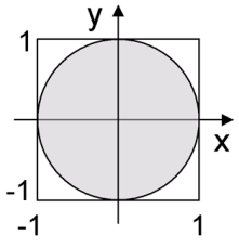
Graphical illustration of rejection sampling. We may compute the area of circle by drawing uniform samples from the square; the fraction of points that fall in the circle represents its area. This method breaks down if the size of the circle is small relative to the size of the square. A special case of Monte Carlo integration is rejection sampling. We may use it to compute the area of a region \(R\) by sampling in a larger region with a known area and recording the fraction of samples that falls within \(R\).

For example, suppose we have a Bayesian network over the set of variables \(X = Z \cup E\). We may use rejection sampling to compute marginal probabilities \(p(E=e)\). We can rewrite the probability as

and then take the Monte Carlo approximation. In other words, we draw many samples from \(p\) and report the fraction of samples that are consistent with the value of the marginal.

Importance sampling

Unfortunately, rejection sampling can be very wasteful. If \(p(E=e)\) equals, say, 1%, then we will discard 99% of all samples.

A better way of computing such integrals uses importance sampling. The main idea is to sample from a distribution \(q\) (hopefully with \(q(x)\) roughly proportional to \(f(x) \cdot p(x)\)), and then reweigh the samples in a principled way, so that their sum still approximates the desired integral.

More formally, suppose we are interested in computing \(\E_{x \sim p}[f(x)]\). We may rewrite this integral as

where \(w(x) = \frac{p(x)}{q(x)}\) and the samples \(x^t\) are drawn from \(q\). In other words, we may instead take samples from \(q\) and reweigh them with \(w(x)\); the expected value of this Monte Carlo approximation will be the original integral.

The variance of this new estimator is

Note that we can set the variance to zero by choosing \(q(x) = \frac{\lvert f(x) \rvert p(x)}{\int \lvert f(x) \rvert p(x) dx}\). If we can sample from this \(q\) (and evaluate the corresponding weight), then we only need a single Monte Carlo sample to compute the true value of our integral. Of course, sampling from such a \(q\) is NP-hard in general (its denominator \(\E_{x \sim p}[\lvert f(x) \vert]\) is basically the quantity we’re trying to estimate in the first place), but this at least gives us an indication for what to strive for.

In the context of our previous example for computing \(p(E=e)\), we may take \(q\) to be the uniform distribution and apply importance sampling as follows:

where \(w_e(z) = p(e, z)/q(z)\). Unlike rejection sampling, this will use all the examples; if \(p(z \mid e)\) is not too far from uniform, this will converge to the true probability after only a very small number of samples.

Normalized importance sampling

Unfortunately, unnormalized importance sampling is not suitable for estimating conditional probabilities of the form

Note that using unnormalized importance sampling, we could estimate the numerator as

where \(\delta(z) = \begin{cases}1 & \text{if $z$ is consistent with $X_i = x_i$} \\ 0 & \text{otherwise}\end{cases}\). The denominator is the same as the result we derived earlier:

If we estimate the numerator \(P(X_i=x_i, E=e)\) and the denominator \(P(E=e)\) with different and independent samples of \(z^t \sim q\), then the errors in the two approximations may compound. For example, if the numerator is an under-estimate and the denominator is an over-estimate, the final probability could be a severe under-estimate.

However, if we use the same set of \(T\) samples \(z^1, \dotsc, z^T \sim q\) for both the numerator and denominator, we avoid this issue of compounding errors. Thus, the final form of normalized importance sampling is

Unfortunately, there is one drawback to the normalized importance sampling estimator, which is that it is biased. If \(T = 1\), then we have

Fortunately, because the numerator and denominator are both unbiased, the normalized importance sampling estimator remains asymptotically unbiased, meaning that

Markov chain Monte Carlo

Let us now turn our attention from computing expectations to performing marginal and MAP inference using sampling. We will solve these problems using a very powerful technique called Markov chain Monte CarloMarkov chain Monte Carlo is another algorithm that was developed during the Manhattan project and eventually republished in the scientific literature some decades later. It is so important, that is was recently named as one of the 10 most important algorithms of the 20th century. (MCMC).

Markov Chain

A key concept in MCMC is that of a Markov chain. A (discrete-time) Markov chain is a sequence of random variables \(S_0, S_1, S_2, \ldots\) with each random variable \(S_i \in \{1,2,\ldots,d\}\) taking one of \(d\) possible values, intuitively representing the state of a system. The initial state is distributed according to a probability \(P(S_0)\); all subsequent states are generated from a conditional probability distribution that depends only on the previous random state, i.e., \(S_i\) is distributed according to \(P(S_i \mid S_{i-1})\).

The probability \(P(S_i \mid S_{i-1})\) is the same at every step \(i\); this means that the transition probabilities at any time in the entire process depend only on the given state and not on the history of how we got there. This is called the Markov assumption.

⊕
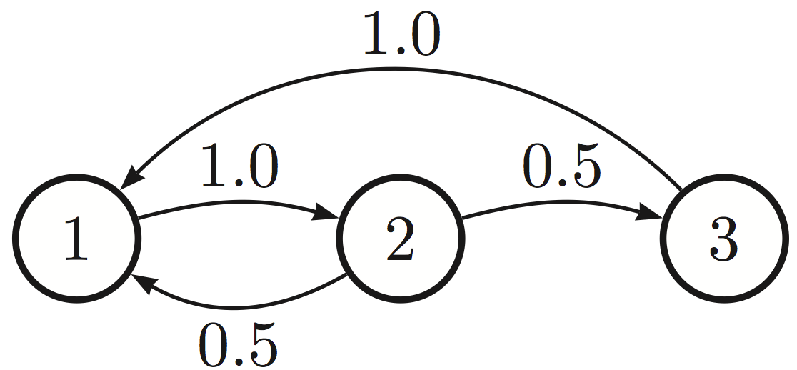
A Markov chain over three states. The weighted directed edges indicate probabilities of transitioning to a different state. It is very convenient to represent the transition probability as a \(d \times d\) matrix

If the initial state \(S_0\) is drawn from a vector probabilities \(p_0\), we may represent the probability \(p_t\) of ending up in each state after \(t\) steps as

where \(T^t\) denotes matrix exponentiation (apply the matrix operator \(t\) times).

The limit \(\pi = \lim_{t \to \infty} p_t\) (when it exists) is called a stationary distribution of the Markov chain. We will construct below Markov chain with a stationary distribution \(\pi\) that exists and is the same for all \(p_0\); we will refer to such \(\pi\) as the stationary distribution of the chain.

A sufficient condition for a stationary distribution is called detailed balance:

It is easy to show that such a \(\pi\) must form a stationary distribution (just sum both sides of the equation over \(x\) and simplify). However, the reverse may not hold and indeed it is possible to have MCMC without satisfying detailed balance.

Existence of a stationary distribution

The high-level idea of MCMC will be to construct a Markov chain whose states will be joint assignments to the variables in the model and whose stationary distribution will equal the model probability \(p\).

In order to construct such a chain, we first need to understand when stationary distributions exist. This turns out to be true under two sufficient conditions:

• Irreducibility: It is possible to get from any state \(x\) to any other state \(x'\) with probability > 0 in a finite number of steps.
• Aperiodicity: It is possible to return to any state at any time, i.e., there exists an \(n\) such that for all \(i\) and all \(n' \geq n\), \(P(s_{n'}=i \mid s_0 = i) > 0\).

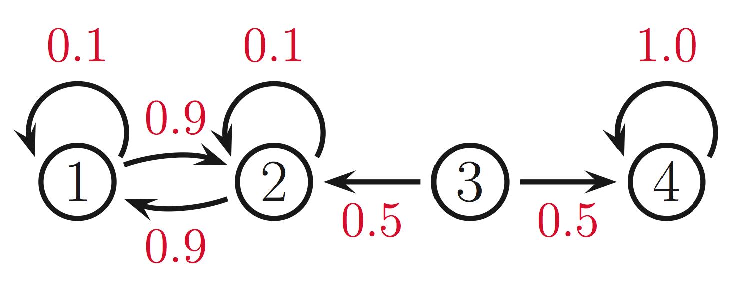
The first condition is meant to prevent absorbing states, i.e., states from which we can never leave. In the example below, if we start in states \(1,2\), we will never reach state 4. Conversely, if we start in state 4, then we will never reach states 1,2. If we start the chain in the middle (in state 3), then clearly it cannot have a single limiting distribution.

The second condition is necessary to rule out transition operators such as

Note that this chain alternates forever between states 1 and 2 without ever settling in a stationary distribution.

Fact: An irreducible and aperiodic finite-state Markov chain has a stationary distribution.

In the context of continuous variables, the Markov chain must be ergodic, which is slightly stronger condition than the above (and which requires irreducibility and aperiodicity). For the sake of generality, we will simply require our Markov Chain to be ergodic.

Markov Chain Monte Carlo

As we said, the idea of MCMC algorithms is to construct a Markov chain over the assignments to a probability function \(p\); the chain will have a stationary distribution equal to \(p\) itself; by running the chain for some number of time, we will thus sample from \(p\).

At a high level, MCMC algorithms will have the following structure. They take as argument a transition operator \(T\) specifying a Markov chain whose stationary distribution is \(p\), and an initial assignment \(x_0\) to the variables of \(p\). An MCMC algorithm then perform the following steps.

1. Run the Markov chain from \(x_0\) for \(B\) burn-in steps.
2. Run the Markov chain for \(N\) sampling steps and collect all the states that it visits.

Assuming \(B\) is sufficiently large, the latter collection of states will form samples from \(p\). We may then use these samples for Monte Carlo integration (or in importance sampling). We may also use them to produce Monte Carlo estimates of marginal probabilities. Finally, we may take the sample with the highest probability and use it as an estimate of the mode (i.e., perform MAP inference).

Metropolis-Hastings algorithm

The Metropolis-Hastings (MH) algorithm is our first way to construct Markov chains within MCMC. The MH method constructs a transition operator \(T(x' \mid x)\) from two components:

• A transition kernel \(Q(x'\mid x)\), specified by the user
• An acceptance probability for moves proposed by \(Q\), specified by the algorithm as

At each step of the Markov chain, we choose a new point \(x'\) according to \(Q\). Then, we either accept this proposed change (with probability \(\alpha\)), or with probability \(1-\alpha\) we remain at our current state.

Notice that the acceptance probability encourages us to move towards more likely points in the distribution (imagine for example that \(Q\) is uniform); when \(Q\) suggests that we move into a low-probability region, we follow that move only a certain fraction of the time.

In practice, the distribution \(Q\) is taken to be something simple, like a Gaussian centered at \(x\) if we are dealing with continuous variables.

Given any \(Q\) the MH algorithm will ensure that \(P\) will be a stationary distribution of the resulting Markov Chain. More precisely, \(P\) will satisfy the detailed balance condition with respect to the MH Markov chain.

To see that, first observe that if \(A(x' \mid x) < 1\), then \(\frac{P(x)Q(x' \mid x)}{P(x')Q(x \mid x')} > 1\) and thus \(A(x \mid x') = 1\). When \(A(x' \mid x) < 1\), this lets us write:

which is simply the detailed balance condition. We used \(T(x \mid x')\) to denote the full transition operator of MH (obtained by applying both \(Q\) and \(A\)). Thus, if the MH Markov chain is ergodic, its stationary distribution will be \(P\).

Gibbs sampling

A widely-used special case of the Metropolis-Hastings methods is Gibbs sampling. Given an ordered set of variables \(x_1,\ldots,x_n\) and a starting configuration \(x^0 = (x_1^0,\ldots,x_n^0)\), consider the following procedure.

Repeat until convergence for \(t = 1, 2,\dots\):

• Set \(x \leftarrow x^{t-1}\).
• For each variable \(x_i\) in the order we fixed:
  1. Sample \(x'_i \sim p(x_i \mid x_{-i})\)
  2. Update \(x \leftarrow (x_1, \dotsc, x'_i, \dotsc, x_n).\)
• Set \(x^t \leftarrow x\)

We use \(x_{-i}\) to denote all variables in \(x\) except \(x_i\). It is often very easy to performing each sampling step, since we only need to condition \(x_i\) on its Markov blanket, which is typically small. Note that when we update \(x_i\), we immediately use its new value for sampling other variables \(x_j\).

Gibbs sampling can be seen as a special case of MH with proposal \(Q(x_i', x_{-i} \mid x_i, x_{-i}) = P(x_i' \mid x_{-i}).\) It is easy check that the acceptance probability simplifies to one.

Assuming the right transition operator, both Gibbs sampling and MH will eventually produce samples from their stationary distribution, which by construction is \(P\).

There exist simple ways of ensuring that this will be the case

• To ensure irreducibility, the transition operator \(Q\) with MH should be able to potentially move to every state. In the case of Gibbs sampling, we would like to make sure that every \(x_i'\) can get sampled from \(p(x_i \mid x_{-i}^t)\).
• To ensure aperiodicity, it is enough to let the chain transition stay in its state with some probability.

In practice, it is not difficult to ensure these requirements are met.

Running time of MCMC

A key parameter to this algorithm in the number of burn-in steps \(B\). Intuitively, this corresponds to the number of steps needed to converge to our limit (stationary) distribution. This is called the mixing time of the Markov chainThere is a technical definition of this quantity, which we will not cover here.. Unfortunately, this time may vary dramatically, and may sometimes take essentially forever. For example, if the transition matrix is

then for small \(\e\) it will take a very long time to reach the stationary distribution, which is close to \((0.5, 0.5)\). At each step, we will stay in the same state with overwhelming probability; very rarely, we will transition to another state, and then stay there for a very long time. The average of these states will converge to \((0.5, 0.5)\), but the convergence will be very slow.

This problem will also occur with complicated distributions that have two distinct and narrow modes; with high probability, the algorithm will sample from a given mode for a very long time. These examples are indications that sampling is a hard problem in general, and MCMC does not give us a free lunch. Nonetheless, for many real-world distributions, sampling will produce very useful solutions.

Another, perhaps more important problem, is that we may not know when to end the burn-in period, even if it is theoretically not too long. There exist many heuristics to determine whether a Markov chain has mixed; however, typically these heuristics involve plotting certain quantities and estimating them by eye; even the quantitative measures are not significantly more reliable than this approach.

In summary, even though MCMC is able to sample from the right distribution (which in turn can be used to solve any inference problem), doing so may sometimes require a very long time, and there is no easy way to judge the amount of computation that we need to spend to find a good solution.