Variable Elimination

Next, we turn our attention to the problem of inference in graphical models. Given a probabilistic model (such as a Bayes net or a MRF), we are interested in using it to answer useful questions, e.g., determining the probability that a given email is spam. More formally, we focus on two types of questions:

Marginal inference: what is the probability of a given variable in our model after we sum everything else out (e.g., probability of spam vs. non-spam)?

\[p(y=1) = \sum_{x_1} \sum_{x_2} \cdots \sum_{x_n} p(y=1, x_1, x_2, \dotsc, x_n).\]

Maximum a posteriori (MAP) inference: what is the most likely assignment to the variables in the model (possibly conditioned on evidence)?

\[\max_{x_1, \dotsc, x_n} p(y=1, x_1, \dotsc, x_n)\]

It turns out that inference is a challenging task. For many probabilities of interest, it is NP-hard to answer any of these questions exactly. Crucially, whether inference is tractable depends on the structure of the graph that describes that probability. If a problem is intractable, we are still able to obtain useful answers via approximate inference methods.

This chapter covers the first exact inference algorithm, variable elimination. We discuss approximate inference in later chapters.

We will assume for the rest of the chapter that $x_i$ are discrete variables taking $k$ possible values eachThe principles behind variable elimination also extend to many continuous distributions (e.g., Gaussians), but we will not discuss these extensions here..

An illustrative example

Consider first the problem of marginal inference. Suppose for simplicity that we are given a chain Bayesian network, i.e., a probability of the form

\[p(x_1, \dotsc, x_n) = p(x_1) \prod_{i=2}^n p(x_i \mid x_{i-1}).\]

We are interested in computing the marginal probability $p(x_n)$. The naive way of calculating this is to sum the probability over all $k^{n-1}$ assignments to $x_1, \dotsc, x_{n-1}$:

\[p(x_n) = \sum_{x_1} \cdots \sum_{x_{n-1}} p(x_1, \dotsc, x_n).\]

However, we can do much better by leveraging the factorization of our probability distribution. We may rewrite the sum in a way that “pushes in” certain variables deeper into the product.

\[\begin{align*} p(x_n) & = \sum_{x_1} \cdots \sum_{x_{n-1}} p(x_1) \prod_{i=2}^n p(x_i \mid x_{i-1}) \\ & = \sum_{x_{n-1}} p(x_n \mid x_{n-1}) \sum_{x_{n-2}} p(x_{n-1} \mid x_{n-2}) \cdots \sum_{x_1} p(x_2 \mid x_1) p(x_1) \end{align*}\]

We sum the inner terms first, starting from $x_1$ and ending with $x_{n-1}$. Concretely, we start by computing an intermediary factor $\tau(x_2) = \sum_{x_1} p(x_2 \mid x_1) p(x_1)$ by summing out $x_1$. This takes $O(k^2)$ time because we must sum over $x_1$ for each assignment to $x_2$. The resulting factor $\tau(x_2)$ can be thought of as a table of $k$ values (though not necessarily probabilities), with one entry for each assignment to $x_2$ (just as factor $p(x_1)$ can be represented as a table). We may then rewrite the marginal probability using $\tau$ as

\[p(x_n) = \sum_{x_{n-1}} p(x_n \mid x_{n-1}) \sum_{x_{n-2}} p(x_{n-1} \mid x_{n-2}) \cdots \sum_{x_2} p(x_3 \mid x_2) \tau(x_2).\]

Note that this has the same form as the initial expression, except that we are summing over one fewer variableThis technique is a special case of dynamic programming, a general algorithm design approach in which we break apart a larger problem into a sequence of smaller ones.. We may therefore compute another factor $\tau(x_3) = \sum_{x_2} p(x_3 \mid x_2) \tau(x_2)$, and repeat the process until we are only left with $x_n$. Since each step takes $O(k^2)$ time, and we perform $O(n)$ steps, inference now takes $O(n k^2)$ time, which is much better than our naive $O(k^n)$ solution.

Also, at each time, we are eliminating a variable, which gives the algorithm its name.

Eliminating Variables

Having established some intuitions, with a special case, we now introduce the variable elimination algorithm in its general form.

Factors

We assume that we are given a graphical model as a product of factors

\[p(x_1, \dotsc, x_n) = \prod_{c \in C} \phi_c(x_c).\]

Recall that we can view a factor as a multi-dimensional table assigning a value to each assignment of a set of variables $x_c$. In a Bayesian network, the factors correspond to conditional probability distributions. In a Markov Random Field, the factors encode an unnormalized distribution; to compute marginals, we first calculate the partition function (also using variable elimination), then we compute marginals using the unnormalized distribution, and finally we divide the result by the partition constant to construct a valid marginal probability.

Factor Operations

The variable elimination algorithm repeatedly performs two factor operations: product and marginalization. We have been implicitly performing these operations in our chain example.

The factor product operation simply defines the product $\phi_3 := \phi_1 \times \phi_2$ of two factors $\phi_1, \phi_2$ as

\[\phi_3(x_c) = \phi_1(x_c^{(1)}) \times \phi_2(x_c^{(2)}).\]

The scope of $\phi_3$ is defined as the union of the variables in the scopes of $\phi_1, \phi_2$; also $x_c^{(i)}$ denotes an assignment to the variables in the scope of $\phi_i$ defined by the restriction of $x_c$ to that scope. For example, we define $\phi_3(a,b,c) := \phi_1(a,b) \times \phi_2(b,c)$.

Next, the marginalization operation “locally” eliminates a set of variables from a factor. If we have a factor $\phi(X,Y)$ over two sets of variables $X,Y$, marginalizing $Y$ produces a new factor

\[\tau(x) = \sum_y \phi(x, y),\]

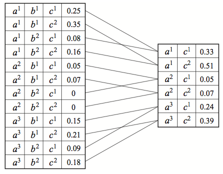
where the sum is over all joint assignments to the set of variables $Y$.⊕ $Here, we are marginalizing out variable $$B$$ from factor $$\phi(A,B,C).$$$
Here, we are marginalizing out variable $B$ from factor $\phi(A,B,C).$

We use $\tau$ to refer to the marginalized factor. It is important to understand that this factor does not necessarily correspond to a probability distribution, even if $\phi$ was a CPD.

Orderings

Finally, the variable elimination algorithm requires an ordering over the variables according to which variables will be “eliminated.” In our chain example, we took the ordering implied by the DAG. It is important to note that:

Different orderings may dramatically alter the running time of the variable elimination algorithm.
It is NP-hard to find the best ordering.

We will come back to these complications later, but for now let the ordering be fixed.

The variable elimination algorithm

We are now ready to formally define the variable elimination (VE) algorithm. Essentially, we loop over the variables as ordered by $O$ and eliminate them in that ordering. Intuitively, this corresponds to choosing a sum and “pushing it in” as far as possible inside the product of the factors, as we did in the chain example.

More formally, for each variable $X_i$ (ordered according to $O$),

Multiply all factors $\Phi_i$ containing $X_i$
Marginalize out $X_i$ to obtain a new factor $\tau$
Replace the factors $\Phi_i$ with $\tau$

A former CS228 student has created an interactive web simulation for visualizing the variable elimination algorithm. Feel free to play around with it and, if you do, please submit any feedback or bugs through the Feedback button on the web app.

Examples

Let’s try to understand what these steps correspond to in our chain example. In that case, the chosen ordering was $x_1, x_2, \dotsc, x_{n-1}$. Starting with $x_1$, we collected all the factors involving $x_1$, which were $p(x_1)$ and $p(x_2 \mid x_1)$. We then used them to construct a new factor $\tau(x_2) = \sum_{x_1} p(x_2 \mid x_1) p(x_1)$. This can be seen as the results of steps 1 and 2 of the VE algorithm: first we form a large factor $\sigma(x_2, x_1) = p(x_2 \mid x_1) p(x_1)$; then we eliminate $x_1$ from that factor to produce $\tau$. Then, we repeat the same procedure for $x_2$, except that the factors are now $p(x_3 \mid x_2), \tau(x_2)$.

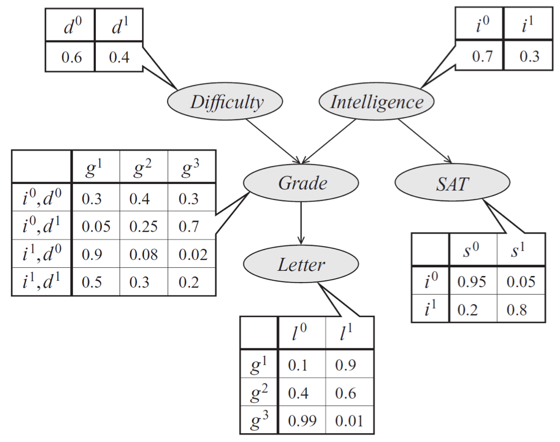
For a slightly more complex example, recall the graphical model of a student’s grade that we introduced earlier.⊕ Bayes net model of a student's grade $$g$$ on an exam; in addition to $$g$$, we also model other aspects of the problem, such as the exam's difficulty $$d$$, the student's intelligence $$i$$, his SAT score $$s$$, and the quality $$l$$ of a reference letter from the professor who taught the course. Each variable is binary, except for $$g$$, which takes 3 possible values.
Bayes net model of a student’s grade $g$ on an exam; in addition to $g$, we also model other aspects of the problem, such as the exam’s difficulty $d$, the student’s intelligence $i$, his SAT score $s$, and the quality $l$ of a reference letter from the professor who taught the course. Each variable is binary, except for $g$, which takes 3 possible values. The probability specified by the model is of the form

\[p(l, g, i, d, s) = p(l \mid g) p(s \mid i) p(i) p(g \mid i, d) p(d).\]

Let’s suppose that we are computing $p(l)$ and are eliminating variables in their topological ordering in the graph. First, we eliminate $d$, which corresponds to creating a new factor $\tau_1(g,i) = \sum_d p(g \mid i, d) p(d)$. Next, we eliminate $i$ to produce a factor $\tau_2(g,s) = \sum_i \tau_1(g,i) p(i) p(s \mid i)$; then we eliminate $s$ yielding $\tau_3(g) = \sum_s \tau_2(g,s)$, and so on. Note that these operations are equivalent to summing out the factored probability distribution as follows:

\[p(l) = \sum_g p(l \mid g) \sum_s \sum_i p(s\mid i) p(i) \sum_d p(g \mid i, d) p(d).\]

Note that this example requires computing at most $k^3$ operations per step, since each factor is at most over 2 variables, and one variable is summed out at each step (the dimensionality $k$ in this example is either 2 or 3).

Introducing evidence

A closely related and equally important problem is computing conditional probabilities of the form

\[P(Y \mid E = e) = \frac{P(Y, E=e)}{P(E=e)}\]

where $P(X,Y,E)$ is a probability distribution, over sets of query variables $Y$, observed evidence variables $E$, and unobserved variables $X$.

We can compute this probability by performing variable elimination once on $P(Y, E=e)$ and then once more on $P(E=e)$.

To compute $P(Y, E=e)$, we simply take every factor $\phi(X', Y', E')$ which has scope over variables $E' \subseteq E$ that are also found in $E$, and we set their values as specified by $e$. Then we perform standard variable elimination over $X$ to obtain a factor over only $Y$.

Running Time of Variable Elimination

It is very important to understand that the running time of Variable Elimination depends heavily on the structure of the graph.

In the previous example, suppose we eliminated $g$ first. Then, we would have had to transform the factors $p(g \mid i, d), \phi(l \mid g)$ into a big factor $\tau(d, i, l)$ over 3 variables, which would require $O(k^4)$ time to compute: $k$ times for each of three conditional variables, and $k$ times for each value of $g$. If we had a factor $S \rightarrow G$, then we would have had to eliminate $p(g \mid s)$ as well, producing a single giant factor $\tau(d, i, l, s)$ in $O(k^5)$ time. Then, eliminating any variable from this factor would require almost as much work as if we had started with the original distribution, since all the variables have become coupled.

Clearly some orderings are more efficient than others. In fact, the running time of Variable Elimination is $O(n k^{M+1})$, where $M$ is the maximum size of any factor $\tau$ formed during the elimination process and $n$ is the number of variables.

Choosing variable elimination orderings

Unfortunately, choosing the optimal VE ordering is an NP-hard problem. However, in practice, we may resort to the following heuristics:

Min-neighbors: Choose a variable with the fewest dependent variables.
Min-weight: Choose variables to minimize the product of the cardinalities of its dependent variables.
Min-fill: Choose vertices to minimize the size of the factor that will be added to the graph.

These methods often result in reasonably good performance in many interesting settings.

Index