Bayesian Learning

The learning approaches we have discussed so far are based on the principle of maximum likelihood estimation. While being extremely general, there are limitations of this approach as illustrated in the two examples below.

Example 1

Let’s suppose we are interested in modeling the outcome of a biased coin, \(X \in \{heads, tails\}\). We toss the coin 10 times, observing 6 heads. If \(\theta\) denotes the probability of observing heads, the maximum likelihood estimate (MLE) is given by,

Now, suppose we continue tossing the coin such that after 100 total trials (including the 10 initial trials), we observe 60 heads. Again, we can compute the MLE as,

In both the above situations, the maximum likelihood estimate does not change as we observe more data. This seems counterintuitive - our confidence in predicting heads with probability 0.6 should be higher in the second setting where we have seen many more trials of the coin! The key problem is that we represent our belief about the probability of heads \(\theta\) as a single number \(\theta_{MLE}\), so there is no way to represent whether we are more or less sure about \(\theta\).

Example 2

Consider a language model for sentences based on the bag-of-words assumption. A bag of words model has a generative process where a sentence is formed from a sample of words which are metaphorically `pulled out of a bag’, i.e. sampled independently. In such a model, the probability of a sentence can be factored as the probability of the words appearing in the sentence, i.e. for a sentence \(S\) consisting of words \(w_1, \ldots, w_n\), we have

For simplicity, assume that our language corpus consists of a single sentence, “Probabilistic graphical models are fun. They are also powerful.” We can estimate the probability of each of the individual words based on the counts. Our corpus contains 10 words with each word appearing once, and hence, each word in the corpus is assigned a probability of 0.1. Now, while testing the generalization of our model to the English language, we observe another sentence, “Probabilistic graphical models are hard.” The probability of the sentence under our model is \(0.1 \times 0.1 \times 0.1 \times 0.1 \times 0 = 0\). We did not observe one of the words (“hard”) during training which made our language model infer the sentence as impossible, even though it is a perfectly plausible sentence.

Out-of-vocabulary words are a common phenomena even for language models trained on large corpus. One of the simplest ways to handle these words is to assign a prior probability of observing an out-of-vocabulary word such that the model will assign a low, but non-zero probability to test sentences containing such words. As an aside, in modern systems, tokenization is commonly used, where a set of fundamental tokens can be combined to form any word. Hence the word “Hello” as a single token and the word “Bayesian” is encoded as “Bay” + “esian” under the common Byte Pair Encoding. This can be viewed as putting a prior over all words, where longer words are less likely.

Setup

In contrast to maximum likelihood learning, Bayesian learning explicitly models uncertainty over both the observed variables \(X\) and the parameters \(\theta\). In other words, the parameters \(\theta\) are random variables as well.

A prior distribution over the parameters, \(p(\theta)\) encodes our initial beliefs. These beliefs are subjective. For example, we can choose the prior over \(\theta\) for a biased coin to be uniform between 0 and 1. If however we expect the coin to be fair, the prior distribution can be peaked around \(\theta = 0.5\). We will discuss commonly used priors later in this chapter.

If we observed the dataset \(\mathcal{D} = \lbrace x_1, \cdots, x_N \rbrace\) (in the coin toss example, each \(X_i\) is the outcome of one toss of the coin) we can update our beliefs using Bayes’ rule,

Hence, Bayesian learning provides a principled mechanism for incorporating prior knowledge into our model. Bayesian learning is useful in many situations such as when want to provide uncertainty estimates about the model parameters (Example 1) or when the data available for learning a model is limited (Example 2).

Conjugate Priors

When calculating posterior distribution using Bayes’ rule, as in the above, it should be pretty straightforward to calculate the numerator. But to calculate the denominator \(p(\mathcal{D})\), we are required to compute an integral

This might cause us trouble, since integration is usually difficult. For this very simple example, we might be able to compute this integral, but as you may have seen many times in this class, if \(\theta\) is high dimensional then computing integrals could be quite challenging.

To tackle this issue, people have observed that for some choices of prior \(p(\theta)\), the posterior distribution \(p(\theta \mid \mathcal{D})\) can be directly computed in closed form. Going back to our coin toss example, where we are given a sequence of \(N\) coin tosses, \(\mathcal{D} = \{x_{1},\ldots,x_{N}\}\) and we want to infer the probability of getting heads \(\theta\) using Bayes rule. Suppose we choose the prior \(p(\theta)\) as the Beta distribution defined by

where \(\alpha_H\) and \(\alpha_T\) are the two parameters that determine the shape of the distribution (similar to how the mean and variance determine a Gaussian distribution), and \(B(\alpha_H, \alpha_T)\) is some normalization constant that ensures \(\int p(\theta)d\theta=1\). We will go into more details about the Beta distribution later. What matters here is that the Beta distribution has a very special property: the posterior \(p(\theta \mid \mathcal{D})\) is always another Beta distribution (but with different parameters). More concretely, out of \(N\) coin tosses, if the number of heads and the number of tails are \(N_H\) and \(N_T\) respectively, then it can be shown that the posterior is:

⊕
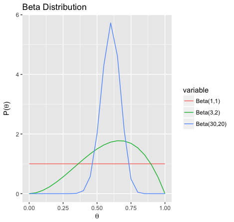
The expectation of both \(\textsf{Beta}(3,2)\) and \(\textsf{Beta}(30,20)\) are \(0.6\), but \(\textsf{Beta}(30,20)\) is much more concentrated. This can be used to represent different levels of uncertainty in \(\theta\)

which is another Beta distribution with parameters \((\alpha_H+N_H, \alpha_T+N_T)\). In other words, if the prior is a Beta distribution (we can represent it as two numbers \(\alpha_H,\alpha_T\)) then the posterior can be immediately computed by a simple addition \(\alpha_H+N_H, \alpha_T+N_T\). There is no need to compute the complex integral \(p(\mathcal{D})\).

Beta Distribution

Now we try to understand the Beta distribution better. If \(\theta\) has distribution \(\textsf{Beta}(\theta \mid \alpha_H, \alpha_T)\), then the expected value of \(\theta\) is \(\frac{\alpha_H}{\alpha_H+\alpha_T}\). Intuitively, \(\alpha_H\) is larger than \(\alpha_T\) if we believe that heads are more likely. The variance of the Beta distribution is the somewhat complex expression \(\frac{\alpha_H\alpha_T}{(\alpha_H+\alpha_T)^2(\alpha_H+\alpha_T+1)}\), but we remark that (very roughly) the numerator is quadratic in \(\alpha_H,\alpha_T\) while the denominator is cubic in \(\alpha_H,\alpha_T\). Hence if \(\alpha_H\) and \(\alpha_T\) are bigger, the variance is smaller, so we are more certain about the value of \(\theta\). We can use this observation to better understand the above posterior update rule: after observing more data \(\mathcal{D}\), the prior parameters \(\alpha_H\) and \(\alpha_T\) increases by \(N_H\) and \(N_T\) respectively. Thus, the variance of \(p(\theta \mid \mathcal{D})\) should be smaller than \(p(\theta)\), i.e. we are more certain about the value of \(\theta\) after observing data \(\mathcal{D}\).

The idea we presented here is usually called “conjugacy”. Using standard terminology, what we have shown here is that the Beta distribution family is a “conjugate prior” to the Bernoulli distribution family. When people say that distribution family A is a conjugate prior to distribution family B, they mean that if \(p(\theta)\) belongs to distribution family A, and \(p(X \mid \theta)\) belongs to distribution family \(B\), then given a dataset of samples \(\mathcal{D} = (x_1, \cdots, x_N)\) the posterior \(p(\theta \mid \mathcal{D})\) is still in distribution family \(A\). Relating this back to the example we have above, if \(p(\theta)\) is a Beta distribution, and \(p(X \mid \theta)\) is a Bernoulli distribution, then \(p(\theta \mid \mathcal{D})\) is still a Beta distribution. In general we usually have a simple algebra expression to compute \(p(\theta \mid \mathcal{D})\) (such as computing \(\alpha_H+N_H, \alpha_T+N_H\) in the example above).

Categorical Distribution

We give another example of a conjugate prior which generalizes the Bernoulli example above. Instead of being limited to binary outcomes, we can now consider the categorical distribution (think of a \(K\)-sided dice). Let \(\mathcal{D} = \{ x_1, \ldots, x_N \}\) be \(N\) rolls of the dice, where \(x_j \in \{ 1, \ldots, K \}\) is the outcome of the \(j\)-th roll. The parameter of the categorical distribution is denoted by \(\theta\)

where \(\sum_{k = 1}^K \theta_k = 1\).

We claim that the Dirichlet distribution is a conjugate prior for the categorical distribution. A Dirichlet distribution is defined by \(K\) parameters \(\mathbf{\alpha} = (\alpha_1, \ldots, \alpha_K)\), and its PDF is given by

where \(B(\alpha)\) is still a normalization constant.

To show that the Dirichlet distribution is a conjugate prior for the categorial distribution, we need to show that the posterior is also a Dirichlet distribution. To calculate the posterior \(p(\theta \mid \mathcal{D})\) with Bayes rule we first calculate the likelihood \(p(\mathcal{D} \mid \theta)\) as

To simply the notation we denote \(N_k = \sum_{j=1}^N 1\lbrace X_j=k\rbrace\) as the number of times we roll out \(k\), so \(p(\mathcal{D}\mid\theta)=\prod\theta_k^{N_k}\). Using this new notation the posterior can be calculated as

In other words, if the prior is a Dirichlet distribution with parameter \((\alpha_1, \cdots, \alpha_K)\) then the posterior \(p(\theta \mid \mathcal{D})\) is a Dirichlet distribution with parameters \((\alpha_1+N_1, \cdots, \alpha_K+N_K)\). In example 2 above, we added a prior probability to observing an out-of-vocabulary word. We can see that this corresponds exactly to choosing a prior with nonzero prior \(\alpha = \alpha_1 = \ldots = \alpha_K\). This is also exactly the same as Laplace smoothing with parameter \(\alpha\). We see that Laplace’s heuristic for handling missing values has a rigorous justification when viewed with the Bayesian formalism.

Some Concluding Remarks

Many distributions have conjugate priors. In fact, any exponential family distribution has a conjugate prior. Even though conjugacy seemingly solves the problem of computing Bayesian posteriors, there are two caveats: 1. Usually practitioners will want to choose the prior \(p(\theta)\) to best capture his or her knowledge about the problem, and using conjugate priors is a strong restriction. 2. For more complex distributions, the posterior computation is not as easy as those in our examples. There are distributions for which the posterior computation is still NP hard.

Conjugate priors is a powerful tool used in many real world applications such as topic modeling (e.g. latent dirichlet allocation) and medical diagnosis. However, practitioners should be mindful of its short-comings and consider and compare with other tools such as MCMC or variational inference (also covered in https://ermongroup.github.io/cs228-notes/inference/sampling/).