Learning in latent variable models

Up to now, we have assumed that when learning a directed or an undirected model, we are given examples of every single variable that we are trying to model.

However, that may not always be the case. Consider for example a probabilistic language model of news articlesA language model $p$ assigns probabilities to sequences of words $x_1,...,x_n$. We can, among other things, sample from $p$ to generate various kinds of sentences.. Each article $x$ typically focuses on a specific topic $t$, e.g., finance, sports, politics. Using this prior knowledge, we may build a more accurate model $p(x \mid t)p(t)$, in which we have introduced an additional, unobserved variable $t$. This model can be more accurate, because we can now learn a separate $p(x \mid t)$ for each topic, rather than trying to model everything with one $p(x)$.

However, since $t$ is unobserved, we cannot directly use the learning methods that we have so far. In fact, the unobserved variables make learning much more difficult; in this chapter, we will look at how to use and how to learn models that involve latent variables.

Latent variable models

More formally, a latent variable model (LVM) $p$ is a probability distribution over two sets of variables $x, z$:

\[p(x, z; \theta),\]

where the $x$ variables are observed at learning time in a dataset $D$ and the $z$ are never observed.

The model may be either directed or undirected. There exist both discriminative and generative LVMs, although here we will focus on the latter (the key ideas hold for discriminative models as well).

Example: Gaussian mixture models

Gaussian mixture models (GMMs) are a latent variable model that is also one of the most widely used models in machine learning. ⊕
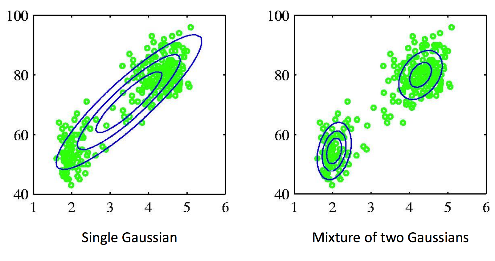
Example of a dataset that is best fit with a mixture of two Gaussians. Mixture models allow us to model clusters in the dataset.

In a GMM, each data point is a tuple $(x_i, z_i)$ with $x_i \in \Re^d$ and $z_i \in \{1, 2, \dotsc, K\}$ ($z_i$ is discrete). The joint $p$ is a directed model

\[p(x, z) = p(x|z)p(z),\]

where $p(z = k) = \pi_k$ for some vector of class probabilities $\pi \in \Delta_{K-1}$ and

\[p(x|z=k) = \mathcal{N}(x; \mu_k, \Sigma_k)\]

is a multivariate Gaussian with mean and variance $\mu_k, \Sigma_k$.

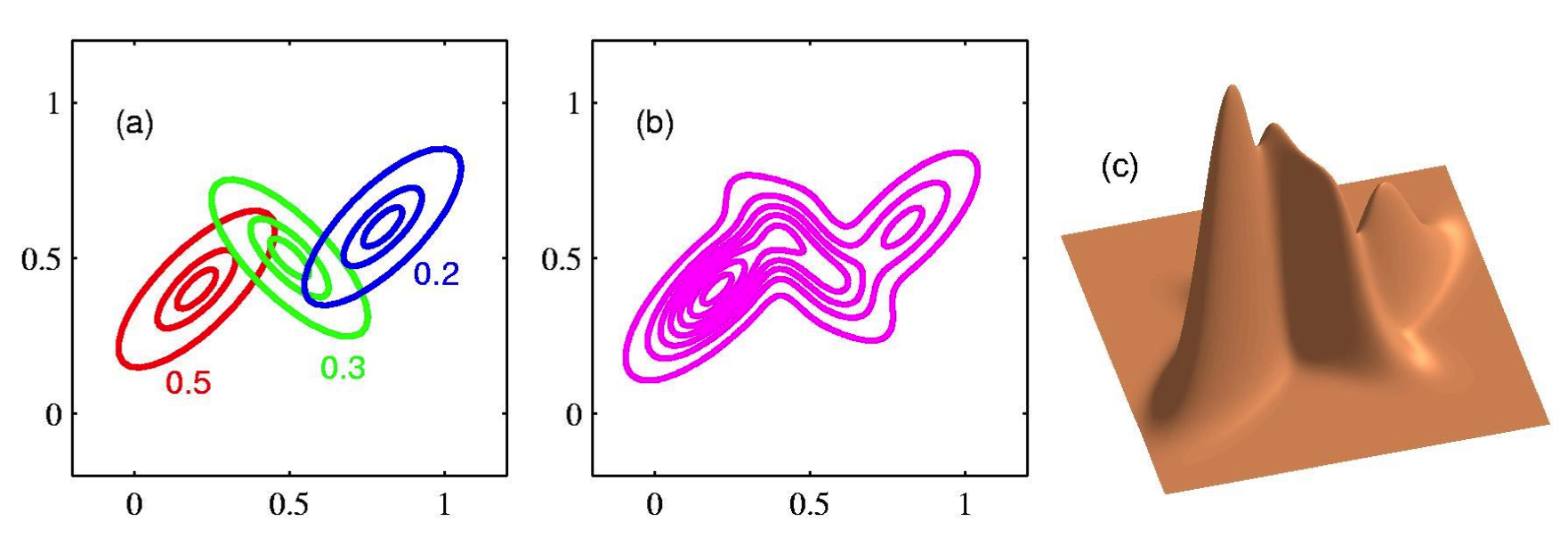
This model postulates that our observed data is comprised of $K$ clusters with proportions specified by $\pi_1, \dotsc, \pi_K$; the distribution within each cluster is a Gaussian. We can see that $p(x)$ is a mixture by explicitly writing out this probability:

\[p(x) = \sum_{k=1}^K p(x|z=k)p(z=k) = \sum_{k=1}^K \pi_k \mathcal{N}(x; \mu_k, \Sigma_k).\]

To generate a new data point, we sample a cluster $k$ and then sample its Gaussian $\mathcal{N}(x; \mu_k, \Sigma_k)$.

Example of a Gaussian mixture model, consisting of three components with different class proportions (a). The true class of each point is unobserved, so the distribution over $$x$$ looks like in (b); it is both multi-modal and non-Gaussian. Visualizing it in 3D shows the effects of class proportions on the magnitudes of the modes.

Why are latent variable models useful?

There are two reasons why we might want to use latent variable models.

The simplest reason is that some data might be naturally unobserved. For example, if we are modeling a clinical trial, then some patients may drop out, and we won’t have their measurements. The methods in this chapter can be used to learn with this kind of missing data.

However, the most important reason for studying LVMs is that they enable us to leverage our prior knowledge when defining a model. Our topic modeling example from the introduction illustrates this. We know that our set of news articles is actually a mixture of $K$ distinct distributions (one for each topic); LVMs allow us to design a model that captures this.

LVMs can also be viewed as increasing the expressive power of our model. In the case of GMMs, the distribution that we can model using a mixture of Gaussian components is much more expressive than what we could have modeled using a single component.

Marginal likelihood training

How do we train an LVM? Our goal is still to fit the marginal distribution $p(x)$ over the visible variables $x$ to that observed in our dataset $D$. Hence our previous discussion about KL divergences applies here as well and by the same argument, we should be maximizing the marginal log-likelihood of the data

\[\log p(D) = \sum_{x \in D} \log p(x) = \sum_{x \in D} \log \left( \sum_z p(x|z) p(z) \right).\]

This optimization objective is considerably more difficult than regular log-likelihood, even for directed graphical models. For one, we can see that the summation inside the log makes it impossible to decompose $p(x)$ into a sum of log-factors. Hence, even if the model is directed, we can no longer derive a simple closed form expression for the parameters.

⊕
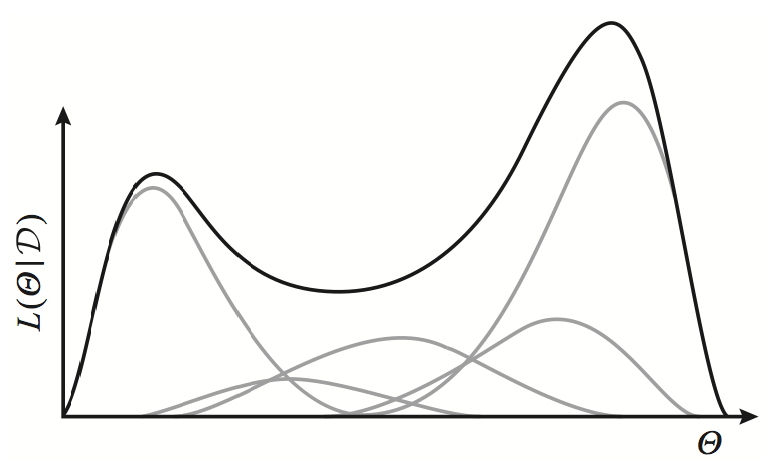
Exponential family distributions (gray lines) have concave log-likelihoods. However, a weighted mixture of such distributions is no longer concave (black line). Looking closer at the distribution of a data point $x$, we also see that it is actually a mixture

\[p(x) = \sum_z p(x|z) p(z)\]

of distributions $p(x \mid z)$ with weights $p(z)$. Whereas a single exponential family distribution $p(x)$ has a concave log-likelihood (as we have seen in our discussion of undirected models), the log of a weighted mixture of such distributions is no longer concave or convex.

This non-convexity requires the development of specialized learning algorithms.

Learning latent variable models

Since the objective is non-convex, we will resort to approximate learning algorithms. These methods are widely used in practice and are quite effectiveNote however, that (quite surprisingly), many latent variable models (like GMMs) admit algorithms that can compute the global optimum of the maximum likelihood objective, even though it is not convex. Such methods are covered at the end of CS229T..

The Expectation-Maximization algorithm

The Expectation-Maximization (EM) algorithm is a hugely important and widely used algorithm for learning directed latent-variable graphical models $p(x,z; \theta)$ with parameters $\theta$ and latent $z$.

The EM algorithm relies on two simple observations.

If the latent $z$ were fully observed, then we could optimize the log-likelihood exactly using our previously seen closed form solution for $p(x,z)$.
Knowing the parameters, we can often efficiently compute the posterior $p(z\mid x; \theta)$ (this is an assumption; it is not true for some models).

EM follows a simple iterative two-step strategy: given an estimate $\theta_t$ of the parameters, compute $p(z\mid x)$ and use it to “hallucinate” values for $z$. Then, find a new $\theta_{t+1}$ by optimizing the resulting tractable objective. This process will eventually converge.

We haven’t exactly defined what we mean by “hallucinating” the data. The full definition is a bit technical, but its instantiation is very intuitive in most models like GMMs.

By “hallucinating” the data, we mean computing the expected log-likelihood

\[\E_{z \sim p(z|x)} \log p(x,z; \theta).\]

This expectation is what gives the EM algorithm half of its name. If $z$ is not too high-dimensional (e.g., in GMMs it is a one-dimensional categorical variable), then we can compute this expectation.

Since the summation is now outside the log, we can maximize the expected log-likelihood. In particular, when $p$ is a directed model, $\log p$ again decomposes into a sum of log-CPD terms that can be optimized independently, as discussed in the chapter on directed graphical models.

We can formally define the EM algorithm as follows. Let $D$ be our dataset.

Starting at an initial $\theta_0$, repeat until convergence for $t = 1, 2, \dotsc$:
E-Step: For each $x \in D$, compute the posterior $p(z\mid x; \theta_t)$.
M-Step: Compute new parameters via

\[\theta_{t+1} = \arg\max_\theta \sum_{x \in D} \E_{z \sim p(z|x; \theta_t)} \log p(x,z; \theta).\]

Example: Gaussian mixture models

Let’s look at this algorithm in the context of GMMs. Suppose we have a dataset $D$. In the E-step, we may compute the posterior for each data point $x$ as follows:

\[p(z \mid x; \theta_t) = \frac{p(z, x; \theta_t)}{p(x; \theta_t)} = \frac{p(x | z; \theta_t) p(z; \theta_t)}{\sum_{k=1}^K p(x | z_k; \theta_t) p(z_k; \theta_t)}.\]

Note that each $p(x \mid z_k; \theta_t) p(z_k; \theta_t)$ is simply the probability that $x$ originates from component $k$ given the current set of parameters $\theta$. After normalization, these form the $K$-dimensional vector of probabilities $p(z \mid x; \theta_t)$.

Recall that in the original model, $z$ is an indicator variable that chooses a component for $x$; we may view this as a “hard” assignment of $x$ to one component. The result of the $E$ step is a $K$-dimensional vector (whose components sum to one) that specifies a “soft” assignment to components. In that sense, we have “hallucinated” a “soft” instantiation of $z$; this is what we meant earlier by an “intuitive interpretation” for $p(z\mid x; \theta_t)$.

At the M-step, we optimize the expected log-likelihood of our model.

\[\begin{align*} \theta_{t+1} & = \arg\max_\theta \sum_{x \in D} \E_{z \sim p(z|x; \theta_t)} \log p(x,z; \theta) \\ & = \arg\max_\theta \sum_{k=1}^K \sum_{x \in D} p(z_k|x; \theta_t) \log p(x|z_k; \theta) + \sum_{k=1}^K \sum_{x \in D} p(z_k|x; \theta_t) \log p(z_k; \theta) \end{align*}\]

We can optimize each of these terms separately. We will start with $p(x\mid z_k; \theta) = \mathcal{N}(x; \mu_k, \Sigma_k)$. We have to find $\mu_k, \Sigma_k$ that maximize

\[\sum_{x \in D} p(z_k|x; \theta_t) \log p(x|z_k; \theta) = c_k \cdot \E_{x \sim Q_k(x)} \log p(x|z_k; \theta),\]

where $c_k = \sum_{x \in D} p(z_k \mid x; \theta_t)$ is a constant that does not depend on $\theta$ and $Q_k(x)$ is a probability distribution defined over $D$ as

\[Q_k(x) = \frac{p(z_k|x; \theta_t)}{\sum_{x \in D} p(z_k|x; \theta_t)}.\]

Now we know that $\E_{x \sim Q_k(x)} \log p(x \mid z_k; \theta)$ is optimized when $p(x \mid z_k; \theta)$ equals $Q_k(x)$ (as discussed in the section on learning directed models, this objective equals the KL divergence between $Q_k$ and $P$, plus a constant). Moreover, since $p(x\mid z_k; \theta) = \mathcal{N}(x; \mu_k, \Sigma_k)$ is in the exponential family, it is entirely described by its sufficient statistics (recall our discussion of exponential families in the section on learning undirected models). Thus, we may set the mean and variance $\mu_k, \Sigma_k$ to those of $Q_k(x)$, which are

\[\mu_k = \mu_{Q_k} = \sum_{x \in D} \frac{ p(z_k|x; \theta_t)}{\sum_{x \in D} p(z_k|x; \theta_t)} x\]

and

\[\Sigma_k = \Sigma_{Q_k} = \sum_{x \in D} \frac{ p(z_k|x; \theta_t)}{\sum_{x \in D} p(z_k|x; \theta_t)} (x-\mu_{Q_k}) (x-\mu_{Q_k})^T.\]

Note how these are the just the mean and variance of the data, weighted by their cluster affinities! Similarly, we may find out that the class priors are

\[\pi_k = \frac{1}{|D|}\sum_{x \in D} p(z_k|x; \theta_t).\]

Although we have derived these results using general facts about exponential families, it’s equally possible to derive them using standard calculus techniques.

EM as variational inference

Why exactly does EM converge? We can understand the behavior of EM by casting it in the framework of variational inference.

Consider the posterior inference problem for $p(z\mid x)$, where the $x$ variables are held fixed as evidence. We may apply our variational inference framework by taking $p(x,z)$ to be the unnormalized distribution; in that case, $p(x)$ will be the normalization constant.

Recall that variational inference maximizes the evidence lower bound (ELBO)

\[\mathcal{L}(p,q) = \E_{q(z)} \left[ \log p(x,z; \theta) - \log q(z) \right]\]

over distributions $q$. The ELBO satisfies the equation

\[\log p(x; \theta) = KL(q(z) \| p(z|x; \theta)) + \mathcal{L}(p,q).\]

Hence, $\mathcal{L}(p,q)$ is maximized when $q=p(z \mid x)$; in that case the KL term becomes zero and the lower bound is tight: $\log p(x; \theta) = \mathcal{L}(p,q).$

The EM algorithm can be seen as iteratively optimizing the ELBO over $q$ (at the E step) and over $\theta$ (at the M) step.

Starting at some $\theta_t$, we compute the posterior $p(z\mid x; \theta)$ at the $E$ step. We evaluate the ELBO for $q = p(z\mid x; \theta)$; this makes the ELBO tight:

\[\log p(x; \theta_t) = \E_{p(z|x; \theta_t)} \log p(x,z; \theta_t) - \E_{p(z|x; \theta_t)} \log p(z|x; \theta_t)\]

Next, we optimize the ELBO over $p$, holding $q$ fixed. We solve the problem

\[\theta_{t+1} = \arg\max_\theta \E_{p(z|x; \theta_t)} \log p(x,z; \theta) - \E_{p(z|x; \theta_t)} \log p(z|x; \theta_t)\]

Note that this is precisely the optimization problem solved at the $M$ step of EM (in the above equation, there is an additive constant independent of $\theta$).

Solving this problem increases the ELBO. However, since we fixed $q$ to $\log p(z\mid x; \theta_t)$, the ELBO evaluated at the new $\theta_{t+1}$ is no longer tight. But since the ELBO was equal to $\log p(x ;\theta_t)$ before optimization, we know that the true log-likelihood $\log p(x;\theta_{t+1})$ must have increased.

We now repeat this procedure, computing $p(z\mid x; \theta_{t+1})$ (the E-step), plugging $p(z\mid x; \theta_{t+1})$ into the ELBO (which makes the ELBO tight), and maximizing the resulting expression over $\theta$. Every step increases the marginal likelihood $\log p(x;\theta_t)$, which is what we wanted to show.

Properties of EM

From our above discussion, it follows that EM has the following properties:

The marginal likelihood increases after each EM cycle.
Since the marginal likelihood is upper-bounded by its true global maximum, and it increases at every step, EM must eventually converge.

However, since we optimizing a non-convex objective, we have no guarantee to find the global optimum. In fact, EM in practice converges almost always to a local optimum, and moreover, that optimum heavily depends on the choice of initialization. Different initial $\theta_0$ can lead to very different solutions, and so it is very common to use multiple restarts of the algorithm and choose the best one in the end. In fact EM is so sensitive to the choice of initial parameters, that techniques for choosing these parameters are still an active area of research.

In summary, the EM algorithm is a very popular technique for optimizing latent variable models that is also often very effective. Its main downside are its difficulties with local minima.

Index