Structure learning for Bayesian networks

The task of structure learning for Bayesian networks refers to learning the structure of the directed acyclic graph (DAG) from data. There are two major approaches for structure learning: score-based and constraint-based.

Score-based approach

The score-based approach first defines a criterion to evaluate how well the Bayesian network fits the data, then searches over the space of DAGs for a structure achieving the maximal score. The score-based approach is essentially a search problem that consists of two parts: the definition of a score metric and the search algorithm.

Score metrics

The score metrics for a structure \(\mathcal{G}\) and data \(D\) can be generally defined as:

Here \(LL(G:D)\) refers to the log-likelihood of the data under the graph structure \(\mathcal{G}\). The parameters in the Bayesian network \(G\) are estimated based on MLE and the log-likelihood score is calculated based on the estimated parameters. If the score function only consisted of the log-likelihood term, then the optimal graph would be a complete graph, which is probably overfitting the data. Instead, the second term \(\phi(\lvert D \rvert) \lVert G \rVert\) in the scoring function serves as a regularization term, favoring simpler models. \(\lvert D \rvert\) is the number of data samples, and \(\|G\|\) is the number of parameters in the graph \(\mathcal{G}\). When \(\phi(t) = 1\), the score function is known as the Akaike Information Criterion (AIC). When \(\phi(t) = \log(t)/2\), the score function is known as the Bayesian Information Criterion (BIC). With the BIC, the influence of model complexity decreases as \(\lvert D \rvert\) grows, allowing the log-likelihood term to eventually dominate the score.

There is another family of Bayesian score function called BD (Bayesian Dirichlet) score. For BD score, it first defines the probability of data \(D\) conditional on the graph structure \(\mathcal{G}\) as

where \(P(D \mid \mathcal{G}, \Theta_{\mathcal{G}})\) is the probability of the data given the network structure and parameters, and \(P(\Theta_{\mathcal{G}} \mid \mathcal{G})\) is the prior probability of the parameters. When the prior probability is specified as a Dirichlet distribution,

Here \(\pi_i\) refers to the parent configuration of the variable \(i\) and \(N_{i,\pi_i,j}\) is the count of variable \(i\) taking value \(j\) with parent configuration \(\pi_i\). \(N'\) represents the counts in the prior respectively.

With a prior for the graph structure \(P(\Theta_{\mathcal{G}})\) (say, a uniform one), the BD score is defined as

Notice there is no penalty term appended to the BD score since it will penalize overfitting implicitly via the integral over the parameter space.

Chow-Liu Algorithm

The Chow-Liu Algorithm is a specific type of score based approach which finds the maximum-likelihood tree-structured graph (i.e., each node has exactly one parent, except for parentless root node). The score is simply the log-likelihood; there is no penalty term for graph structure complexity since the algorithm only considers tree structures.

The algorithm has three steps:

1. Compute the mutual information for all pairs of variables \(X,U\), and form a complete graph from the variables where the edge between variables \(X,U\) has weight \(MI(X,U)\):

   \[MI(X,U) =\sum_{x,u} \hat p(x,u)\log\left[\frac{\hat p(x,u)}{\hat p(x) \hat p(u)}\right]\]

   This function measures how much information \(U\) provides about \(X\). The graph with computed MI edge weights might resemble:

   

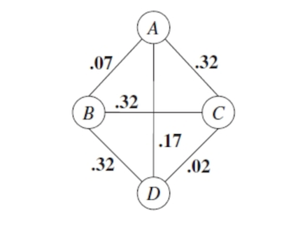
   Remember that from our empirical distribution \(\hat p(x,u) = \frac{Count(x,u)}{\# \text{ data points}}\).

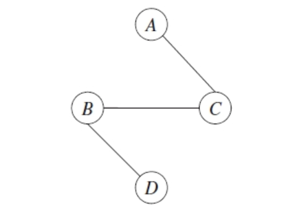
2. Find the maximum weight spanning tree: the maximal-weight tree that connects all vertices in a graph. This can be found using Kruskal or Prim Algorithms.

   

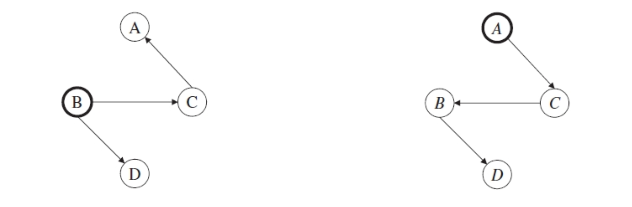
3. Pick any node to be the root variable, and assign directions radiating outward from this node (arrows go away from it). This step transforms the resulting undirected tree to a directed one.

   

The Chow-Liu Algorithm has a complexity of order \(n^2\), as it takes \(O(n^2)\) to compute mutual information for all pairs, and \(O(n^2)\) to compute the maximum spanning tree.

Having described the algorithm, let’s explain why this works. It turns out that the likelihood score decomposes into mutual information and entropy terms:

We would like to find a graph \(G\) that maximizes this log-likelihood. Since the entropies are independent of the dependency ordering in the tree, the only terms that change with the choice of \(G\) are the mutual information terms. So we want

Now if we assume \(G = (V,E)\) is a tree (where each node has at most one parent), then

The orientation of edges does not matter because mutual information is symmetric. Thus we can see why the Chow-Liu algorithm finds a tree-structure that maximizes the log-likelihood of the data.

Search algorithms

The most common choice for search algorithms are local search and greedy search.

For local search algorithm, it starts with an empty graph or a complete graph. At each step, it attempts to change the graph structure by a single operation of adding an edge, removing an edge or reversing an edge. (Of course, the operation should preserve the acyclic property.) If the score increases, then it adopts the attempt and does the change, otherwise it makes another attempt.

For greedy search (namely the K3 algorithm), we first assume a topological order of the graph. For each variable, we restrict its parent set to the variables with a higher order. While searching for parent set for each variable, it takes a greedy approach by adding the parent that increases the score most until no improvement can be made.

A former CS228 student has created an interactive web simulation for visualizing the K3 learning algorithm. Feel free to play around with it and, if you do, please submit any feedback or bugs through the Feedback button on the web app.

Although both approaches are computationally tractable, neither of them have a guarantee of the quality of the graph that we end up with. The graph space is highly “non-convex” and both algorithms might get stuck at some sub-optimal regions.

Constraint-based approach

The constraint-based case employs the independence test to identify a set of edge constraints for the graph and then finds the best DAG that satisfies the constraints. For example, we could distinguish V-structure and fork-structure by doing an independence test for the two variables on the sides conditional on the variable in the middle. This approach works well with some other prior (expert) knowledge of structure but requires lots of data samples to guarantee testing power. So it is less reliable when the number of sample is small.

Recent Advances

In this section, we will briefly introduce two recent algorithms for graph search: order-search (OS) approach and integer linear programming (ILP) approach.

The OS approach, as its name suggests, conducts a search over the topological orders and the graph space at the same time. The K3 algorithm assumes a topological order in advance and searches only over the graphs that obey the topological order. When the order specified is a poor one, it may end with a bad graph structure (with a low graph score). The OS algorithm resolves this problem by performing a search over orders at the same time. It swaps the order of two adjacent variables at each step and employs the K3 algorithm as a sub-routine.

The ILP approach encodes the graph structure, scoring and the acyclic constraints into a linear programming problem. Thus it can utilize a state-of-art integer programming solver. That said, this approach requires a bound on the maximum number of parents any node in the graph can have (say to be 4 or 5). Otherwise, the number of constraints in the ILP will explode and the computation will become intractable.