Introduction

Probabilistic graphical modeling is a branch of machine learning that studies how to use probability distributions to describe the world and to make useful predictions about it.

There are dozens of reasons to learn about probabilistic modeling. For one, it is a fascinating scientific field with a beautiful theory that bridges in surprising ways two very different branches of mathematics: probability and graph theory. Probabilistic modeling also has intriguing connections to philosophy, particularly the question of causality.

At the same time, probabilistic modeling is widely used throughout machine learning and in many real-world applications. These techniques can be used to solve problems in fields as diverse as medicine, language processing, vision, and many others.

This combination of elegant theory and powerful applications makes graphical models one of the most fascinating topics in modern artificial intelligence and computer scienceThe 2011 Turing award (considered to be the “Nobel prize of computer science”) was recently awarded to Judea Pearl for founding the field of probabilistic graphical modeling..

Probabilistic modeling

But what is, exactly, probabilistic modeling? When trying to solve a real-world problem using mathematics, it is very common to define a mathematical model of the world in the form of an equation. Perhaps the simplest model would be a linear equation of the form

\[y = \beta^T x,\]

where $y$ is an outcome variable that we want to predict, and $x$ are known (given) variables that affect the outcome. For example, $y$ may be the price of a house, and $x$ are a series of factors that affect this price, e.g., the location, the number of bedrooms, the age of the house, etc. We assume that $y$ is a linear function of this input (parameterized by $\beta$).

Often, the real world that we are trying to model is very complicated; in particular, it often involves a significant amount of uncertainty (e.g., the price of a house has a certain chance of going up if a new subway station opens within a certain distance). It is therefore very natural to deal with this uncertainty by modeling the world in the form of a probability distributionFor a more philosophical discussion of why one should use probability theory as opposed to something else, see the Dutch book argument for probabilism.

\[p(x,y).\]

Given such a model, we could ask questions such as “what is the probability that house prices will rise over the next five years?”, or “given that the house costs $100,000, what is the probability that it has three bedrooms?” The probabilistic aspect of modeling is very important, because:

Typically, we cannot perfectly predict the future. We often don’t have enough knowledge about the world, and often the world itself is stochastic.
We need to assess the confidence of our predictions; often, predicting a single value is not enough, we need the system to output its beliefs about what’s going on in the world.

In this course, we will study principled ways of reasoning about uncertainty and use ideas from both probability and graph theory to derive efficient machine learning algorithms for this task. We will find answers to many interesting questions, such as:

What are the tradeoffs between computational complexity and the richness of a probabilistic model?
What is the best model for inferring facts about the future, given a fixed dataset and computational budget?
How does one combine prior knowledge with observed evidence in a principled way to make predictions?
How can we rigorously analyze whether $A$ is the cause of $B$, or vice versa?

In addition, we will also see many examples of how to apply probabilistic techniques to various problems, such as disease prediction, image understanding, language analysis, etc.

The difficulties of probabilistic modeling

To get a first taste of the challenges that lie ahead of us, consider a simple application of probabilistic modeling: spam classification.

Suppose we have a model $\pt(y, x_1, \dotsc, x_n)$ of word occurrences in spam and non-spam mail. Each binary variable $x_i$ encodes whether the $i$-th English word is present in the email; the binary variable $y$ indicates whether the email is spam. In order to classify a new email, we may look at the probability $P(y=1 \mid x_1, \dotsc, x_n)$.

What is the “size” of the function $\pt$ that we just defined? Our model defines a probability in $[0,1]$ for each combination of inputs $y, x_1, \dotsc, x_n$; specifying all these probabilities will require us to write down a staggering $2^{n+1}$ different values, one for each assignment to our $n+1$ binary variables. Since $n$ is the size of the English vocabulary, this is clearly impractical from both a computational (how do we store this large list?) and from a statistical (how do we efficiently estimate the parameters from limited data?) point of view. More generally, our example illustrates one of the main challenges that this course will deal with: probabilities are inherently exponentially-sized objects; the only way in which we can manipulate them is by making simplifying assumptions about their structure.

The main simplifying assumption that we will make in this course is that of conditional independence among the variables. For example, suppose that the English words are all conditionally independent given $Y$. In other words, the probabilities of seeing two words are independent given that a message is spam. This is clearly an oversimplification, as the probabilities of the words “pills” and “buy” are clearly correlated; however, for most words (e.g., “penguin” and “muffin”) the probabilities will indeed be independent, and our assumption will not significantly degrade the accuracy of the model.

We refer to this particular choice of independencies as the Naive Bayes assumption. Given this assumption, we can write the model probability as a product of factors

\[P(y, x_1, \dotsc, x_n) = p(y) \prod_{i=1}^n p(x_i \mid y).\]

Each factor $p(x_i \mid y)$ can be completely described by a small number of parameters (4 parameters with 2 degrees of freedom to be exact). The entire distribution is parametrized by $O(n)$ parameters, which we can tractably estimate from data and make predictions.

Describing probabilities with graphs

Our independence assumption can be conveniently represented in the form of a graph.⊕
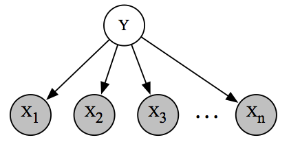
Graphical representation of the Naive Bayes spam classification model. We can interpret the directed graph as indicating a story of how the data was generated: first, a spam/non-spam label was chosen at random; then a subset of $n$ possible English words were sampled independently and at random. This representation has the immediate advantage of being easy to understand. It can be interpreted as telling us a story: an email was generated by first choosing at random whether the email is spam or not (indicated by $y$), and then by sampling words one at a time. Conversely, if we have a story of how our dataset was generated, we can naturally express it as a graph with an associated probability distribution.

More importantly, we want to submit various queries to the model (e.g., what is the probability of spam given that I see the word “pill”?); answering these questions will require specialized algorithms that will be most naturally defined using graph-theoretical concepts. We will also use graph theory to analyze the speed of learning algorithms and to quantify the computational complexity (e.g., NP-hardness) of different learning tasks.

The take-away point we want to get across is that there is an intimate connection between probability distributions and graphs that will be exploited throughout the course for defining, learning, and working with probabilistic models.

A bird’s eye overview of the course

Our discussion of graphical models will be divided into three major parts: representation (how to specify a model), inference (how to ask the model questions), and learning (how to fit a model to real-world data). These three themes will also be closely linked: to derive efficient inference and learning algorithms, the model will need to be adequately represented; furthermore, learning models will require inference as a subroutine. Thus, it will be best to always keep the three tasks in mind, rather than focusing on them in isolationFor a more detailed overview, see this writeup by Neal Parikh; this part of the notes is based on it..

Representation

How do we express a probability distribution that models some real-world phenomenon? This is not a trivial problem: we have seen that a naive model for classifying spam messages with $n$ possible words requires us in general to specify $O(2^n)$ parameters. We will address this difficulty via general techniques for constructing tractable models. These recipes will make heavy use of graph theory; probabilities will be described by graphs whose properties (e.g., connectivity, tree-width) will reveal probabilistic and algorithmic features of the model (e.g., independence, learning complexity).

Inference

Given a probabilistic model, how do we obtain answers to relevant questions about the world? Such questions often reduce to querying the marginal or conditional probabilities of certain events of interest. More concretely, we will be typically interested in asking the system two types of questions:

Marginal inference: what is the probability of a given variable in our model after we sum everything else out? An example query would be to determine the probability that a random house has more than three bedrooms.

\[p(x_1) = \sum_{x_2} \sum_{x_3} \cdots \sum_{x_n} p(x_1, x_2, \dotsc, x_n).\]

Maximum a posteriori (MAP) inference asks for the most likely assignment of variables. For example, we may try to determine the most likely spam message, solving the problem

\[\underset{x_1, \dots, x_n}{\operatorname{argmax}}p(x_1,\dotsc,x_n, y=1).\]

Often our queries will involve evidence (like in the MAP example above), in which case we will fix the assignment of a subset of the variables.

It turns out that inference is a very challenging task. For many probabilities of interest, it will be NP-hard to answer any of these questions. Crucially, whether inference is tractable will depend on the structure of the graph that describes that probability! If a problem is intractable, we will still be able to obtain useful answers via approximate inference methods. Interestingly, algorithms described in this part of the course will be heavily based on work done in the statistical physics community in the mid-20th century.

Learning

Our last key task refers to fitting a model to a dataset, which could be for example a large number of labeled examples of spam. By looking at the data, we can infer useful patterns (e.g., which words are found more frequently in spam emails), which we can then use to make predictions about the future. However, we will see that learning and inference are also inherently linked in a more subtle way, since inference will turn out to be a key subroutine that we will repeatedly call within learning algorithms. Also, the topic of learning will feature important connections to the field of computational learning theory — which deals with questions such as generalization from limited data and overfitting — as well as to Bayesian statistics — which tells us (among other things) about how to combine prior knowledge and observed evidence in a principled way.

Index