Bayesian networks

We begin with the topic of representation: how do we choose a probability distribution to model some interesting aspect of the world? Coming up with a good model is not always easy: we have seen in the introduction that a naive model for spam classification would require us to specify a number of parameters that is exponential in the number of words in the English language!

In this chapter, we will learn about one way to avoid these kinds of complications. We are going to:

• Learn an effective and general technique for parameterizing probability distributions using only a few parameters.
• See how the resulting models can be elegantly described via directed acyclic graphs (DAGs).
• Study connections between the structure of a DAG and the modeling assumptions made by the distribution that it describes; this will not only make these modeling assumptions more explicit, but will also help us design more efficient inference algorithms.

The kinds of models that we will see here are referred to as Bayesian networks. In the next chapter, we will also see a second approach, which involves undirected graphs, also known as Markov random fields (MRFs). Bayesian networks effectively show causality, whereas MRFs cannot. Thus, MRFs are preferable for problems where there is no clear causality between random variables.

Probabilistic modeling with Bayesian networks

Directed graphical models (a.k.a. Bayesian networks) are a family of probability distributions that admit a compact parametrization that can be naturally described using a directed graph.

The general idea behind this parametrization is surprisingly simple.

Recall that by the chain rule, we can write any probability \(p\) as:

A compact Bayesian network is a distribution in which each factor on the right hand side depends only on a small number of ancestor variables \(x_{A_i}\):

For example, in a model with five variables, we may choose to approximate the factor \(p(x_5 \mid x_4, x_3, x_2, x_1)\) with \(p(x_5 \mid x_4, x_3)\). In this case, we write \(x_{A_5} = \{x_4, x_3\}\).

When the variables are discrete (which will often be the case in the problems we will consider), we may think of the factors \(p(x_i\mid x_{A_i})\) as probability tables, in which rows correspond to assignments to \(x_{A_i}\) and columns correspond to values of \(x_i\); the entries contain the actual probabilities \(p(x_i\mid x_{A_i})\). If each variable takes \(d\) values and has at most \(k\) ancestors, then the entire table will contain at most \(O(d^{k+1})\) entries. Since we have one table per variable, the entire probability distribution can be compactly described with only \(O(nd^{k+1})\) parameters (compared to \(O(d^n)\) with a naive approach).

Graphical representation.

Distributions of this form can be naturally expressed as directed acyclic graphs, in which vertices correspond to variables \(x_i\) and edges indicate dependency relationships. In particular we set the parents of each node \(x_i\) to its ancestors \(x_{A_i}\).

As an example, consider a model of a student’s grade \(g\) on an exam. This grade depends on the exam’s difficulty \(d\) and the student’s intelligence \(i\); it also affects the quality \(l\) of the reference letter from the professor who taught the course. The student’s intelligence \(i\) affects the SAT score \(s\) as well. Each variable is binary, except for \(g\), which takes 3 possible values.⊕
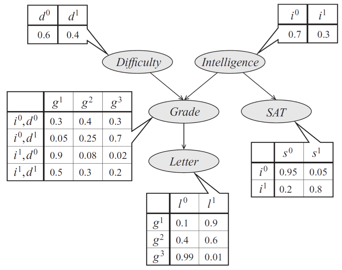
Bayes net model describing the performance of a student on an exam. The distribution can be represented a product of conditional probability distributions specified by tables. The form of these distributions is described by edges in the graph. The joint probability distribution over the 5 variables naturally factorizes as follows:

The graphical representation of this distribution is a DAG that visually specifies how random variables depend on each other. The graph clearly indicates that the letter depends on the grade, which in turn depends on the student’s intelligence and the difficulty of the exam.

Another way to interpret directed graphs is in terms of stories for how the data was generated. In the above example, to determine the quality of the reference letter, we may first sample an intelligence level and an exam difficulty; then, a student’s grade is sampled given these parameters; finally, the recommendation letter is generated based on that grade.

In the previous spam classification example, we implicitly postulated that email is generated according to a two-step process: first, we choose a spam/non-spam label \(y\); then we sample independently whether each word is present, conditioned on that label.

Formal definition.

Formally, a Bayesian network is a directed graph \(G = (V,E)\) together with

• A random variable \(x_i\) for each node \(i \in V\).
• One conditional probability distribution (CPD) \(p(x_i \mid x_{A_i})\) per node, specifying the probability of \(x_i\) conditioned on its parents’ values.

Thus, a Bayesian network defines a probability distribution \(p\). Conversely, we say that a probability \(p\) factorizes over a DAG \(G\) if it can be decomposed into a product of factors, as specified by \(G\).

It is not hard to see that a probability represented by a Bayesian network will be valid: clearly, it will be non-negative and one can show using an induction argument (and using the fact that the CPDs are valid probabilities) that the sum over all variable assignments will be one. Conversely, we can also show by counter-example that when \(G\) contains cycles, its associated probability may not sum to one.

The dependencies of a Bayes net

To summarize, Bayesian networks represent probability distributions that can be formed via products of smaller, local conditional probability distributions (one for each variable). By expressing a probability in this form, we are introducing into our model assumptions that certain variables are independent.

This raises the question: which independence assumptions are we exactly making by using a Bayesian network model with a given structure described by \(G\)? This question is important for two reasons: we should know precisely what model assumptions we are making (and whether they are correct); also, this information will help us design more efficient inference algorithms later on.

Let us use the notation \(I(p)\) to denote the set of all independencies that hold for a joint distribution \(p\). For example, if \(p(x,y) = p(x) p(y)\), then we say that \(x \perp y \in I(p)\).

Independencies described by directed graphs

It turns out that a Bayesian network \(p\) very elegantly describes many independencies in \(I(p)\); these independencies can be recovered from the graph by looking at three types of structures.

For simplicity, let’s start by looking at a Bayes net \(G\) with three nodes: \(X\), \(Y\), and \(Z\). In this case, \(G\) essentially has only three possible structures, each of which leads to different independence assumptions. The interested reader can easily prove these results using a bit of algebra.

• ⊕
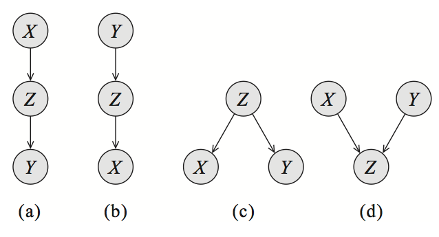
  Bayesian networks over three variables, encoding different types of dependencies: cascade (a,b), common parent (c), and v-structure (d). Common parent. If \(G\) is of the form \(X \leftarrow Z \rightarrow Y\), and \(Z\) is observed, then \(X \perp Y \mid Z\). However, if \(Z\) is unobserved, then \(X \not\perp Y\). Intuitively this stems from the fact that \(Z\) contains all the information that determines the outcomes of \(X\) and \(Y\); once it is observed, there is nothing else that affects these variables’ outcomes.
• Cascade: If \(G\) equals \(X \rightarrow Z \rightarrow Y\), and \(Z\) is again observed, then, again \(X \perp Y \mid Z\). However, if \(Z\) is unobserved, then \(X \not\perp Y\). Here, the intuition is again that \(Z\) holds all the information that determines the outcome of \(Y\); thus, it does not matter what value \(X\) takes.
• V-structure (also known as explaining away): If \(G\) is \(X \rightarrow Z \leftarrow Y\), then knowing \(Z\) couples \(X\) and \(Y\). In other words, \(X \perp Y\) if \(Z\) is unobserved, but \(X \not\perp Y \mid Z\) if \(Z\) is observed.

The latter case requires additional explanation. Suppose that \(Z\) is a Boolean variable that indicates whether our lawn is wet one morning; \(X\) and \(Y\) are two explanations for it being wet: either it rained (indicated by \(X\)), or the sprinkler turned on (indicated by \(Y\)). If we know that the grass is wet (\(Z\) is true) and the sprinkler didn’t go on (\(Y\) is false), then the probability that \(X\) is true must be one, because that is the only other possible explanation. Hence, \(X\) and \(Y\) are not independent given \(Z\).

These structures clearly describe the independencies encoded by a three-variable Bayesian net. We can extend them to general networks by applying them recursively over any larger graph. This leads to a notion called \(d\)-separation (where \(d\) stands for directed).

Let \(Q\), \(W\), and \(O\) be three sets of nodes in a Bayesian Network \(G\). We say that \(Q\) and \(W\) are \(d\)-separated given \(O\) (i.e. the variables \(O\) are observed) if \(Q\) and \(W\) are not connected by an active path. An undirected path in \(G\) is called active given observed variables \(O\) if for every consecutive triple of variables \(X,Y,Z\) on the path, one of the following holds:

• \(X \leftarrow Y \leftarrow Z\), and \(Y\) is unobserved \(Y \not\in O\)
• \(X \rightarrow Y \rightarrow Z\), and \(Y\) is unobserved \(Y \not\in O\)
• \(X \leftarrow Y \rightarrow Z\), and \(Y\) is unobserved \(Y \not\in O\)
• \(X \rightarrow Y \leftarrow Z\), and \(Y\) or any of its descendants are observed. ⊕
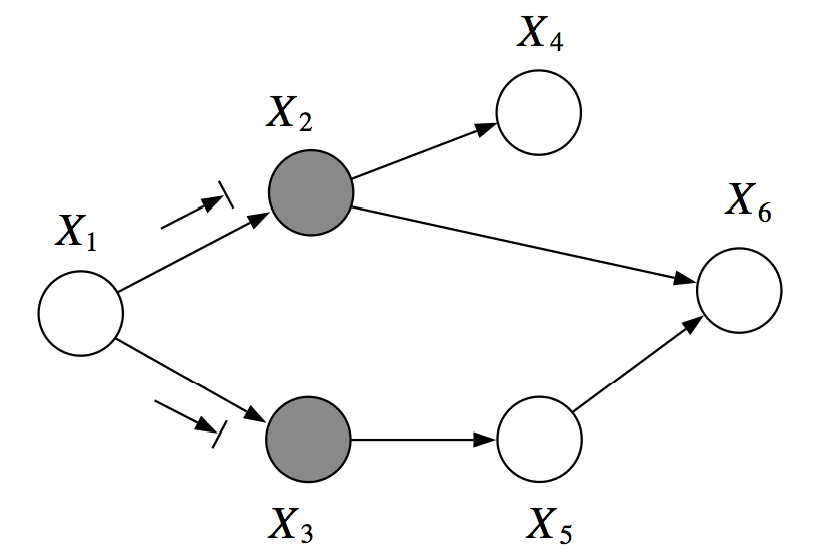
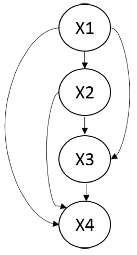
  In this example, \(X_1\) and \(X_6\) are \(d\)-separated given \(X_2, X_3\). ⊕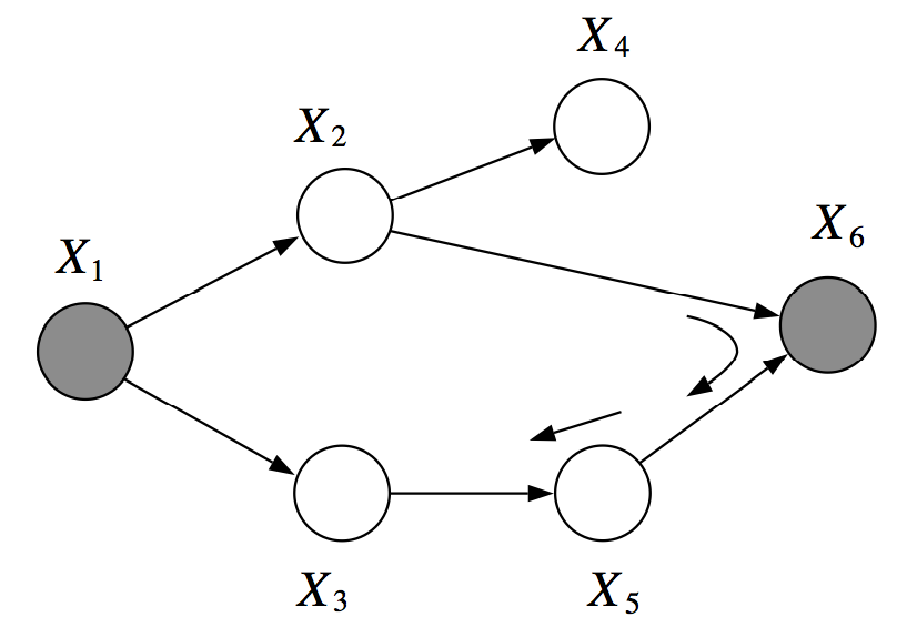
  However, \(X_2, X_3\) are not \(d\)-separated given \(X_1, X_6\). There is an active pass which passed through the V-structure created when \(X_6\) is observed.

For example, in the graph below, \(X_1\) and \(X_6\) are \(d\)-separated given \(X_2, X_3\). However, \(X_2, X_3\) are not \(d\)-separated given \(X_1, X_6\), because we can find an active path \((X_2, X_6, X_5, X_3)\)

A former CS228 student has created an interactive web simulation for testing \(d\)-separation. Feel free to play around with it and, if you do, please submit any feedback or bugs through the Feedback button on the web app.

The notion of \(d\)-separation is useful, because it lets us describe a large fraction of the dependencies that hold in our model. Let \(I(G) = \{(X \perp Y \mid Z) : \text{$X,Y$ are $d$-sep given $Z$}\}\) be a set of variables that are \(d\)-separated in \(G\).

FactWe will not formally prove this, but the intuition is that if \(X,Y\) and \(Y,Z\) are mutually dependent, so are \(X,Z\). Thus we can look at adjacent nodes and propagate dependencies according to the local dependency structures outlined above.: If \(p\) factorizes over \(G\), then \(I(G) \subseteq I(p)\). In this case, we say that \(G\) is an \(I\)-map (independence map) for \(p\).

In other words, all the independencies encoded in \(G\) are sound: variables that are \(d\)-separated in \(G\) are truly independent in \(p\). However, the converse is not true: a distribution may factorize over \(G\), yet have independencies that are not captured in \(G\).

In a way this is almost a trivial statement. If \(p(x,y) = p(x)p(y)\), then this distribution still factorizes over the graph \(y \rightarrow x\), since we can always write it as \(p(x,y) = p(x\mid y)p(y)\) with a CPD \(p(x\mid y)\) in which the probability of \(x\) does not actually vary with \(y\). However, we can construct a graph that matches the structure of \(p\) by simply removing that unnecessary edge.

The representational power of directed graphs

This raises our last and perhaps most important question: can directed graphs express all the independencies of any distribution \(p\)? More formally, given a distribution \(p\), can we construct a graph \(G\) such that \(I(G) = I(p)\)?

First, note that it is easy to construct a \(G\) such that \(I(G) \subseteq I(p)\). A fully connected DAG \(G\) is an \(I\)-map for any distribution since \(I(G) = \emptyset\). ⊕
A fully connected Bayesian network over four variables. There are no independencies in this model, and it is an \(I\)-map for any distribution.

A more interesting question is whether we can find a minimal \(I\)-map \(G\) for \(p\), i.e. an \(I\)-map \(G\) such that the removal of even a single edge from \(G\) will result in it no longer being an \(I\)-map. This is quite easy: we may start with a fully connected \(G\) and remove edges until \(G\) is no longer an \(I\)-map. One way to do this is by following the natural topological ordering of the graph, and removing node ancestors until this is no longer possible; we will revisit this pruning method towards the end of course when performing structure learning.

However, what we are truly interested in determining is whether any probability distribution \(p\) always admits a perfect map \(G\) for which \(I(p)=I(G)\). Unfortunately, the answer is no. For example, consider the following distribution \(p\) over three variables \(X,Y,Z\): we sample \(X,Y \sim \text{Ber}(0.5)\) from a Bernoulli distribution, and we set \(Z = X \text{ xor } Y\) (we call this the noisy-xor example). One can check using some algebra \(\{X \perp Y, Z \perp Y, X \perp Z\} \in I(p)\) but \(Z \perp \{Y,X\} \not\in I(p)\). Thus, \(X \rightarrow Z \leftarrow Y\) is an \(I\)-map for \(p\), but none of the 3-node graph structures that we discussed perfectly describes \(I(p)\), and hence this distribution doesn’t have a perfect map.

A related question is whether perfect maps are unique when they exist. Again, this is not the case, as \(X \rightarrow Y\) and \(X \leftarrow Y\) encode the same independencies, yet form different graphs. More generally, we say that two Bayes nets \(G_1, G_2\) are \(I\)-equivalent if they encode the same dependencies \(I(G_1) = I(G_2)\).

When are two Bayesian nets \(I\)-equivalent? To answer this, let’s return to a simple example with three variables. Each of the graphs below have the same skeleton, meaning that if we drop the directionality of the arrows, we obtain the same undirected graph in each case.

The cascade-type structures (a,b) are clearly symmetric and the directionality of arrows does not matter. In fact, (a,b,c) encode exactly the same dependencies. We can change the directions of the arrows as long as we don’t turn them into a V-structure (d). When we do have a V-structure, however, we cannot change any arrows: structure (d) is the only one that describes the dependency \(X \not\perp Y \mid Z\). These examples provide intuition for the following general result on \(I\)-equivalence.

Fact: If \(G,G'\) have the same skeleton and the same v-structures, then \(I(G) = I(G').\)

Again, it is easy to understand intuitively why this is true. Two graphs are \(I\)-equivalent if the \(d\)-separation between variables is the same. We can flip the directionality of any edge, unless it forms a v-structure, and the \(d\)-connectivity of the graph will be unchanged. We refer the reader to the textbook of Koller and Friedman for a full proof in Theorem 3.7 (page 77).