Inference - random walk satisfiability solvers

Introduction

So far, we’ve introduced propositional logic and considered the problem of deciding whether a propositional formula is satisfiable. The algorithms we’ve studied so far to decide satisfiability, such as DPLL and CDCL, are algorithms which conduct a systematic search of the state space, terminating only when the algorithm has found a satisfying assignment or a proof that the formula is unsatisfiable.

In this lecture, we’ll introduce a randomized algorithm for deciding whether a propositional formula is satisfiable or not, which returns a correct answer with high probability. Instead of systematically searching the state space, we’ll conduct a random walk over the state space which can then be analyzed using Markov chains.

The setup for the random walk is as follows. Given a formula with $n$ Boolean variables, define our state space to consist of all possible truth assignments to these $n$ Boolean variables. By considering a mapping from $n$ truth assignments to binary strings of length $n$, our state space can be equivalently viewed as a Boolean hypercube of dimension $n$, where each of the $2^{n}$ vertices corresponds to a truth assignment. Later, we will set up a randomized search procedure which does a random walk over the possible states to decide whether a formula is satisfiable. This type of search is known as a stochastic local search procedure.

Review of Markov chains

A Markov chain is a discrete stochastic process $(X_{n},n\geq0)$ where each $X_{n}\in S$ ($S$ is the state space). A Markov chain satisfies the Markov property, the key conditional independence relationship: the future is conditionally independent of the past given the present. Explicitly, we can write this as $P(X_{n+1}=j\mid X_{n}=i,...,X_{0}=i_{0})=P(X_{n+1}=j\mid X_{n}=i)$ for all possible states $j,i_{0},...i$ and all time steps $n$.

Furthermore, if $P(X_{n+1}=j\mid X_{n}=i)=P_{ij}$ holds for all $n$, then the transition probabilities are independent of time, and we call the Markov chain homogenous. In this case, we can define the transition matrix $P=[P_{ij}]$, and the full joint probability distribution defined by the Markov chain is then completely determined by the transition matrix $P$ and the initial probability distribution $\Pi^{0}$.

Graphically, we can represent a Markov chain as a directed graph with weighted edges. Each node in the graph represents a possible state of the Markov chain. We have directed edges between nodes with edges weights representing the probability of transitioning between the corresponding states.

Random walk algorithm for 2-SAT

Let the state space $S=\{0,1\}^{n}$ be the set of vertices of the Boolean hypercube. Since the number of possible states is $2^{n}$, for large $n$, the state space cannot be enumerated completely, and the transition matrix $P$ cannot be represented explicitly. We want to find a way to simulate from the Markov chain without representing the Markov chain explicitly.

We’ll first consider the following algorithm for solving 2-CNF formulas (a CNF formula where every clause has at most 2 variables) and then generalize later.

Input: a 2-CNF formula with $n$ variables

1. Repeat $b$ times:
   1. Pick an arbitrary truth assignment $x$
   2. Repeat $2n^{2}$ times:
      1. If $x$ satisfies all clauses, return satisfiable
      2. Otherwise, pick any clause that is not satisfied and choose one of the variables uniformly at random from this clause and flip the truth assignment of that variable
2. Return unsatisfiable

Analysis of algorithm for 2-SAT

If the propositional formula is unsatisfiable, then the algorithm will always return unsatisfiable. If the formula is satisfiable, then the algorithm might not find the satisfying assignment. This is the only case where the algorithm makes a mistake. We’ll bound the error probability for this case.

Let $a=a_{1}...a_{n}$ be a truth value assignment which satisfies the CNF formula. Let $x_{t}$ be the truth assignment in the $t^{th}$ iteration of the inner loop. Define the random variable $X_{t}$ to be the number of bits for which $x_{t}$ and $a$ match. If $X_{t}=n$, then we’ve found the satisfying assignment $a$.

Note that when we flip any one bit in $x_{t}$, $X_{t}$ either increases or decreases by 1. Thus, in the inner loop when we flip the truth assignment of some variable, if $X_{t}=j$, then $X_{t+1}$ can only take on the values $\{j-1,j+1\}$.

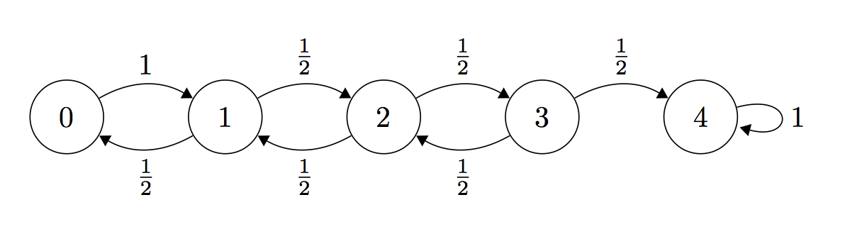
To analyze the transition probabilities, note that when we pick a violated clause in the inner loop, we know that the truth assignment for at least one of the variables in that clause does not match the corresponding truth assignment in $a$ (because $a$ is a satisfying assignment). In either the case where one of the variables is set incorrectly or both of the variables are set incorrectly, the following inequalities hold for the transition probabilities:

$\begin{eqnarray*} P[X_{t+1}=j+1\mid X_{t}=j] & \geq & \frac{1}{2}\\ P[X_{t+1}=j-1\mid X_{t}=j] & \leq & \frac{1}{2} \end{eqnarray*} \ $

for any $1\leq j\leq n-1$ and all time steps $t$. For the boundary cases, we have that $P[X_{t+1}=1\mid X_{t}=0]=1$ and $P[X_{t+1}=n\mid X_{t}=n]=1$ for all $t$.

Thus, we see that the random walk algorithm defines a stochastic process with a Markov chain over the random variable $\{X_{t}\}$, where each $X_{t}\in\{0,...,n\}$. For the purposes of our analysis, we will treat the transition probabilities as exactly $\frac{1}{2}$ which give us a bound on the worst-case performance.

Define $y_{j}=$ # of steps to reach state $n$ from state $j$, and define $h_{j}=E[y_{j}]$. Note that the variables take on the boundary values $h_{n}=0$ and $h_{0}=1+h_{1}$. The expected number of steps are related via the formula:

$\begin{eqnarray*} E[y_{j}] & = & \frac{1}{2}{\left(1+E[y_{j-1}]\right)}+\frac{1}{2}{\left(1+E[y_{j+1}]\right)}\\ h_{j} & = & \frac{h_{j-1}+h_{j+1}}{2}+1 \end{eqnarray*} \ $

Claim 1: $h_{j}=h_{j+1}+2j+1$

Proof: Define $f_{j}=h_{j}-h_{j-1}$. From the recurrence relation above, we have that $f_{j+1}=f_{j}-2$. Since $f_{1}=-1$ by the boundary condition, it follows that $f_{j+1}=-(2j+1)$.

Claim 2: $h_{j}=n^{2}-j^{2}$

Proof: Since $h_{n}=0$ by the boundary condition, it follows from repeated application of Claim 1 that $h_{j}=\sum_{i=j}^{n-1}(2i+1)$.

Thus, we see that if the formula is satisfiable, the random walk will take, in expectation, roughly $n^{2}$ steps to find the satisfying assignment $a$. Let $Z=$ number of steps the random walk takes before reaching state $n$. By Markov’s inequality, $P[Z\geq2n^{2}]\leq\frac{1}{2}$, so the probability that the random walk does not find the satisfying assignment $a$ in $2n^{2}$ steps is $\leq\frac{1}{2}$. By running many independent runs of this algorithm, the failure probability for this random walk algorithm can be lowered to at most ${\left(\frac{1}{2}\right)}^{b}$. Thus, we see that this random walk algorithm provably solves 2-SAT in polynomial time.

Random walk algorithm for 3-SAT

Last lecture, we described and analyzed a random walk algorithm for deciding whether or not a 2-CNF formula is satisfiable. Now consider running the same algorithm presented last time on a 3-CNF formula. We’ll see later on in this lecture why we choose to repeat the inner loop $3n$ times and always generate our truth assignment $x$ uniformly at random.

Input: a 3-CNF formula $\phi(x_{1},...,x_{n})$

1. Repeat $b$ times:
   1. Select truth assignment $x$ uniformly at random
   2. Repeat $3n$ times:
      1. If $x$ satisfies all clauses in $\phi$, return satisfiable
      2. Otherwise, pick any clause that is not satisfied and choose one of the variables uniformly at random from this clause and flip the truth assignment of that variable
2. Return unsatisfiable

Analysis of algorithm for 3-SAT

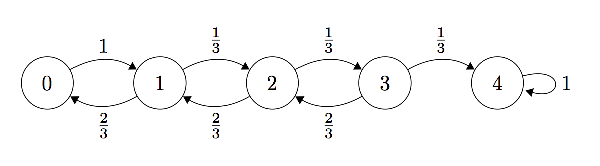
Using a similar analysis as in the last lecture, the bounds for the transition probabilities become

$\begin{eqnarray*} P[X_{t+1}=j+1\mid X_{t}=j] & \geq & \frac{1}{3}\\ P[X_{t+1}=j-1\mid X_{t}=j] & \leq & \frac{2}{3} \end{eqnarray*} \ $

for any $1\leq j\leq n-1$ and all time steps $t$. For the boundary cases, we have that $P[X_{t+1}=1\mid X_{t}=0]=1$ and $P[X_{t+1}=n\mid X_{t}=n]=1$ for all $t$.

Define $y_{j}=$ # of steps to reach state $n$ from state $j$, and define $h_{j}=E[y_{j}]$. Note that the variables take on the boundary values $h_{n}=0$ and $h_{0}=1+h_{1}$. The expected number of steps are related via the formula:

$\begin{eqnarray*} h_{j} & = & \frac{2}{3}h_{j-1}+\frac{1}{3}h_{j+1}+1\\ \end{eqnarray*} \ $

Define $f_{j}=h_{j}-h_{j-1}$. From the recurrence relation above, we have that $f_{j+1}=2f_{j}-3$. Since $f_{1}=-1$ by the boundary condition, $-f_{j}=O(2^{j})$. Therefore, $h_{j-1}=h_{j}+O(2^{j})$, and this gives us a biased random walk where $h_{j}=O(2^{n})$.

If we work out the terms explicitly, we have that $h_{j}=2^{n+2}-2^{j+2}-3(n-j)$. Note that even $h_{n-1}=2^{n+2}-2^{n+1}-3=O(2^{n})$. This means that even if we were only one state away from finding the satisfying assignment, the expected running time is still exponential. This observation motivates the following modification to our algorithm.

Suppose that we have a way of starting the Markov chain at state $n-1$. Then instead of simulating the Markov chain for an exponential number of steps hoping to find the satisfying assignment, the best approach is to continually restart the Markov chain at state $n-1$ and just take 1 step at a time until we find the satisfying assignment. We will extend this idea to our algorithm by using very aggressive random restarts and short random walks.

To start, recall that our algorithm will select a truth assignment $x$ uniformly at random. The probability that our initial assignment will have $j$ of the $n$ truth assignments assigned correctly is $P(X_{0}=j)=\frac{1}{2^{n}}{n \choose j}$.

Consider a short sequence of moves and let us compute the probability that if we make $2k+j$ moves, we have $k$ moves to the left and $k+j$ moves to the right: ${2k+j \choose k}{\left(\frac{2}{3}\right)}^{k}{\left(\frac{1}{3}\right)}^{k+j}$.

Now suppose we start at state $n-j$. Let us work out a lower bound for $q_{j}$, the probability of reaching state $n$, starting at state $n-j$, in $\leq3n$ moves. In particular, $q_{j}\geq$ probability that if we make $3j$ moves, we have $j$ moves to the left and $2j$ moves to the right. Using the formula above, we have that $q_{j}\geq{3j \choose j}{\left(\frac{2}{3}\right)}^{j}{\left(\frac{1}{3}\right)}^{2j}$.

By Stirling’s approximation, $n!\sim\sqrt{2\pi n}{\left(\frac{n}{e}\right)}^{n}$ so

$\begin{eqnarray*} {3j \choose j} & = & \frac{(3j)!}{(2j)!j!}\\ & \geq & \frac{c\sqrt{2\pi3j}}{\sqrt{2\pi j}\sqrt{2\pi2j}}{\left(\frac{3j}{e}\right)}^{3j}{\left(\frac{e}{2j}\right)}^{2j}{\left(\frac{e}{j}\right)}^{j}\\ & = & \frac{a}{\sqrt{j}}{\left(\frac{27}{4}\right)}^{j} \end{eqnarray*} \ $

for $j>0$. Combining this bound with our previous expression, $q_{j}\geq\frac{a}{\sqrt{j}}{\left(\frac{1}{2}\right)}^{j}$ for $j>0$. The boundary condition is $q_{0}=1$.

Combining everything, the probability that we will reach state $n$, starting from a truth assignment initialized uniformly at random, in $\leq3n$ moves is

$\begin{eqnarray*} q & \geq & \sum_{j=0}^{n}P(X_{0}=n-j)q_{j}\\ & \geq & \frac{1}{2^{n}}+\sum_{j=1}^{n}\frac{1}{2^{n}}{n \choose j}{\left(\frac{a}{\sqrt{j}}\frac{1}{2^{j}}\right)}\\ & \geq & \frac{1}{2^{n}}+\frac{1}{2^{n}}\frac{a}{\sqrt{n}}\sum_{j=1}^{n}{n \choose j}\frac{1}{2^{j}}\\ & \approx & \frac{a}{\sqrt{n}}{\left(\frac{3}{4}\right)}^{n} \end{eqnarray*} \ $

Therefore, the expected number of times that we have to repeat the procedure before getting a success is $\frac{1}{q}\leq\frac{\sqrt{n}}{a}{\left(\frac{4}{3}\right)}^{n}$. Choose $b=\frac{2}{q}$. Then our algorithm succeeds with probability at least $1/2$ with running time $O{\left(\big(\frac{4}{3}\big)^{n}\right)}$. We can finally boost our algorithm to the desired success probability. In conclusion, we’ve seen that we can go from a biased random walk with $h_{j}=O(2^{n})$ to an expected run time of $O{\left(\big(\frac{4}{3}\big)^{n}\right)}$ by using very aggressive random restarts.

Other variants

WalkSAT

WalkSAT is similar to the random walk algorithm described above. The difference is that when trying to fix a violated clause, WalkSAT will be greedy with some probability.

After selecting a clause $c$,

1. With probability $p$, pick a variable in $c$ at random and flip the truth assignment of $c$
2. Otherwise, go through all the variables in $c$ and choose the variable with the smallest break count to flip (number of satisfied clauses that become unsatisfied when the variable is flipped).

GSAT

1. With probability $p$, choose a variable at random and flip the truth assignment
2. Otherwise, check all variables $x_{1}...x_{n}$ and select the variable with largest ${\Delta}=$ make count - break count

Simulated annealing

1. Randomly pick a variable, calculate ${\Delta}E=$ make count - break count
2. If the new state is a better state (lower energy), always make the transition
3. Otherwise, accept the transition with probability $p=\exp{\left(\frac{-{\Delta}E}{T}\right)}$ where T is the temperature parameter

Note that the randomness helps the algorithm not get trapped in local minima.