Variational inference

In the last chapter, we saw that inference in probabilistic models is often intractable, and we learned about algorithms that provide approximate solutions to the inference problem (e.g., marginal inference) by using subroutines that involve sampling random variables. Most sampling-based inference algorithms are instances of Markov Chain Monte-Carlo (MCMC); two popular MCMC methods are Gibbs sampling and Metropolis-Hastings.

Unfortunately, these sampling-based methods have several important shortcomings.

• Although they are guaranteed to find a globally optimal solution given enough time, it is difficult to tell how close they are to a good solution given the finite amount of time that they have in practice.
• In order to quickly reach a good solution, MCMC methods require choosing an appropriate sampling technique (e.g., a good proposal in Metropolis-Hastings). Choosing this technique can be an art in itself.

In this chapter, we are going to look at an alternative approach to approximate inference called the variational family of algorithms.

Inference as optimization

The main idea of variational methods is to cast inference as an optimization problem.

Suppose we are given an intractable probability distribution \(p\). Variational techniques will try to solve an optimization problem over a class of tractable distributions \(\mathcal{Q}\) in order to find a \(q \in \mathcal{Q}\) that is most similar to \(p\). We will then query \(q\) (rather than \(p\)) in order to get an approximate solution.

The main differences between sampling and variational techniques are that:

• Unlike sampling-based methods, variational approaches will almost never find the globally optimal solution.
• However, we will always know if they have converged. In some cases, we will even have bounds on their accuracy.
• In practice, variational inference methods often scale better and are more amenable to techniques like stochastic gradient optimization, parallelization over multiple processors, and acceleration using GPUs.

Although sampling methods were historically invented first (in the 1940s), variational techniques have been steadily gaining popularity and are currently the more widely used inference technique.

The Kullback-Leibler divergence

To formulate inference as an optimization problem, we need to choose an approximating family \(\mathcal{Q}\) and an optimization objective \(J(q)\). This objective needs to capture the similarity between \(q\) and \(p\); the field of information theory provides us with a tool for this called the Kullback-Leibler (KL) divergence.

Formally, the KL divergence between two distributions \(q\) and \(p\) with discrete support is defined as

In information theory, this function is used to measure differences in information contained within two distributions. The KL divergence has the following properties that make it especially useful in our setting:

• \(KL(q\|p) \geq 0\) for all \(q,p\).
• \(KL(q\|p) = 0\) if and only if \(q = p\).

These can be proven as an exercise. Note however that \(KL(q\|p) \neq KL(p\|q)\), i.e., the KL divergence is not symmetric. This is why we say that it’s a divergence, but not a distance. We will come back to this distinction shortly.

The variational lower bound

How do we perform variational inference with a KL divergence? First, let’s fix a form for \(p\). We’ll assume that \(p\) is a general (discrete, for simplicity) undirected model of the form

where the \(\phi_k\) are the factors and \(Z(\theta)\) is the normalization constant. This formulation captures virtually all the distributions in which we might want to perform approximate inference, such as marginal distributions of directed models \(p(x\mid e) = p(x,e)/p(e)\) with evidence \(e\).

Given this formulation, optimizing \(KL(q\|p)\) directly is not possible because of the potentially intractable normalization constant \(Z(\theta)\). In fact, even evaluating \(KL(q\|p)\) is not possible, because we need to evaluate \(p\).

Instead, we will work with the following objective, which has the same form as the KL divergence, but only involves the unnormalized probability \(\tp(x) = \prod_{k} \phi_k(x_k; \theta)\):

This function is not only tractable, it also has the following important property:

Since \(KL(q\|p) \geq 0\), we get by rearranging terms that

Thus, \(-J(q)\) is a lower bound on the log partition function \(\log Z(\theta)\). In many cases, \(Z(\theta)\) has an interesting interpretation. For example, we may be trying to compute the marginal probability \(p(x \mid D) = p(x,D) / p(D)\) of variables \(x\) given observed data \(D\) that plays the role of evidence. We assume that \(p(x,D)\) is directed. In this case, minimizing \(J(q)\) amounts to maximizing a lower bound on the log-likelihood \(\log p(D)\) of the observed data.

Because of this property, \(-J(q)\) is called the variational lower bound or the evidence lower bound (ELBO); it is often written in the form

Crucially, the difference between \(\log Z(\theta)\) and \(-J(q)\) is precisely \(KL(q\|p)\). Thus, by maximizing the evidence-lower bound, we are minimizing \(KL(q\|p)\) by “squeezing” it between \(-J(q)\) and \(\log Z(\theta)\).

On the choice of KL divergence

To recap, we have just defined an optimization objective for variational inference (the variational lower bound) and we have shown that maximizing the lower bound leads to minimizing the divergence \(KL(q\|p)\).

Recall how we said earlier that \(KL(q\|p) \neq KL(p\|q)\); both divergences equal zero when \(q = p\), but assign different penalties when \(q \neq p\). This raises the question: why did we choose one over the other and how do they differ?

Perhaps the most important difference is computational: optimizing \(KL(q\|p)\) involves an expectation with respect to \(q\), while \(KL(p\|q)\) requires computing expectations with respect to \(p\), which is typically intractable even to evaluate.

However, choosing this particular divergence affects the returned solution when the approximating family \(\mathcal{Q}\) does not contain the true \(p\). Observe that \(KL(q\|p)\) — which is called the I-projection or information projection — is infinite if \(p(x) = 0\) and \(q(x) > 0\):

This means that if \(p(x) = 0\) we must have \(q(x) = 0\). We say that \(KL(q\|p)\) is zero-forcing for \(q\) and it will typically under-estimate the support of \(p\).

On the other hand, \(KL(p\|q)\) — known as the M-projection or the moment projection — is infinite if \(q(x) = 0\) and \(p(x) > 0\). Thus, if \(p(x) > 0\) we must have \(q(x) > 0\). We say that \(KL(p\|q)\) is zero-avoiding for \(q\) and it will typically over-estimate the support of \(p\).

The figure below illustrates this phenomenon graphically.

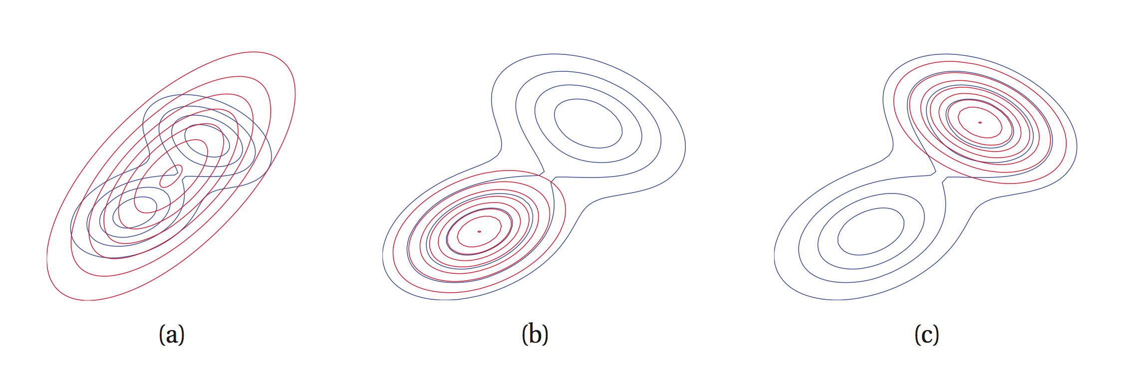
Due to the properties that we just described, we often call \(KL(p\|q)\) the inclusive KL divergence, while \(KL(q\|p)\) is the exclusive KL divergence.

Mean-field inference

The next step in our development of variational inference concerns the choice of approximating family \(\mathcal{Q}\). The machine learning literature contains dozens of proposed ways to parametrize this class of distributions; these include exponential families, neural networks, Gaussian processes, latent variable models, and many others types of models.

However, one of the most widely used classes of distributions is simply the set of fully-factored \(q(x) = q_1(x_1) q_2(x_2) \cdots q_n(x_n)\); here each \(q_i(x_i)\) is categorical distribution over a one-dimensional discrete variable, which can be described as a one-dimensional table.

This choice of \(\mathcal{Q}\) turns out to be easy to optimize over and works surprisingly well. It is perhaps the most popular choice when optimizing the variational bound; variational inference with this choice of \(\mathcal{Q}\) is called mean-field inference. It consists in solving the following optimization problem:

The standard way of performing this optimization problem is via coordinate descent over the \(q_j\): we iterate over \(j=1,2,\ldots,n\) and for each \(j\) we optimize \(KL(q\|p)\) over \(q_j\) while keeping the other “coordinates” \(q_{-j} = \prod_{i \neq j} q_i\) fixed.

Interestingly, the optimization problem for one coordinate has a simple closed form solution:

Notice that both sides of the above equation contain univariate functions of \(x_j\): we are thus replacing \(q(x_j)\) with another function of the same form. The constant term is a normalization constant for the new distribution.

Notice also that on right-hand side, we are taking an expectation of a sum of factors

Of these, only factors belonging to the Markov blanket of \(x_j\) are a function of \(x_j\) (simply by the definition of the Markov blanket); the rest are constant with respect to \(x_j\) and can be pushed into the constant term.

This leaves us with an expectation over a much smaller number of factors; if the Markov blanket of \(x_j\) is small (as is often the case), we are able to analytically compute \(q(x_j)\). For example, if the variables are discrete with \(K\) possible values, and there are \(F\) factors and \(N\) variables in the Markov blanket of \(x_j\), then computing the expectation takes \(O(K F K^N)\) time: for each value of \(x_j\) we sum over all \(K^N\) assignments of the \(N\) variables, and in each case, we sum over the \(F\) factors.

The result of this is a procedure that iteratively fits a fully-factored \(q(x) = q_1(x_1) q_2(x_2) \cdots q_n(x_n)\) that approximates \(p\) in terms of \(KL(q\|p)\). After each step of coordinate descent, we increase the variational lower bound, tightening it around \(\log Z(\theta)\).

In the end, the factors \(q_j(x_j)\) will not quite equal the true marginal distributions \(p(x_j)\), but they will often be good enough for many practical purposes, such as determining \(\max_{x_j} p(x_j)\).