TL;DR: Objectives based on maximum likelihood and adversarial training are widely used for learning generative models but rarely compared in a rigorous, quantitative way. We propose a new approach to evaluate, compare, and interpolate between these two learning paradigms. We find that even though adversarial training generates visually appealing samples, it shows a strong preference for distributions of “small” support which manifests as extremely poor likelihood values – even a trivial Gaussian mixture model memorizing the training data achieves better likelihoods (and beautiful samples)! A hybrid objective interpolating between maximum likelihood and adversarial training attains a fine balance between competitive likelihoods and sample quality metrics.

At its very core, the goal of any generative model is to approximate a data distribution as closely as possible. Yet, the following fundamental question is still largely open:

Given a parametric family of models, how should we measure (and optimize) closeness between the model distribution and the data distribution?

Accordingly, many learning principles have been proposed for learning generative models (Mohamed and Lakshminarayanan 2016). Here, we focus on two predominant paradigms: maximum likelihood estimation and adversarial training.

Maximum likelihood estimation

As the name suggests, the idea is to pick the parameters that maximize the probability (likelihood) of observing the data. Going back to the idea of measuring closeness, it turns out this objective is equivalent to minimizing the Kullback-Liebler (KL) divergence between the data distribution and the model distribution. Maximum likelihood estimators are statistically efficient under certain conditions, and a variety of probabilistic models are learned by directly optimizing likelihood or its approximations.

These include undirected models such as restricted Boltzmann Machines (Hinton 2002) as well as directed models such as autoregressive models (Larochelle and Murray 2011), variational autoencoders (Kingma and Welling 2014), and normalizing flow models (Dinh, Krueger, and Bengio 2014; Dinh, Sohl-Dickstein, and Bengio 2017). However, evaluation and/or optimization of the likelihood of a model may not always be tractable. In such cases, a common resort is approximate inference techniques. For example, restricted Boltzmann Machines are often trained by approximating gradients of the log-likelihood using Markov chain Monte Carlo, whereas variational autoencoders (VAE) introduce variational approximations to the posterior and optimize a stochastic lower bound to the log-likelihood. Alternatively, adversarial training is a learning objective that is likelihood-free, i.e., it does not explicitly involve a likelihood function, and can therefore avoid some of the above difficulties.

Adversarial training

In adversarial training, we seek a generative model that can produce (by sampling) data that is indistinguishable from the data used for training. In particular, generative adversarial networks (Goodfellow et al. 2014) use an auxilliary binary classifier to distinguish between real training data and samples from the model. The parameters of the classifier and the generative model are optimized using a minimax (adversarial) objective where the classifier is trying to distinguish the samples as well as it can, and the generator is trying to fool the classifier.¹

Learning such models can hence sidestep the evaluation and optimization of an explicit likelihood function, but requires the ability to efficiently sample from the model distribution. The latter is true for directed probabilistic models which allow for efficient ancestral sampling.

An apples vs. oranges apples comparison

A key question to ask is which of these two learning principles, maximum likelihood or adversarial training, is a better candidate for learning generative models. A comparison of maximum likelihood and adversarial training is ill-posed without defining a uniform set of evaluation metrics and modeling assumptions.

Evaluation metrics

Held-out likelihoods is a natural metric, especially for models learned using the maximum likelihood principle. Recall that our setup assumes access to a data distribution only via samples (as opposed to an analytical expression). Hence for the purpose of evaluation of generalization performance (and hyperparameter optimization), we can construct multiple empirical estimates of the data distribution. In the case of models learned using maximum likelihood, this is analogous to constructing a training, validation, and test set whereby the generative model is trained to minimize the KL divergence with respect to an empirical data distribution defined by the training set, hyperparameters are optimized based on likelihoods assigned by the model on the validation set, and finally generalization is evaluated based on the likelihoods asssigned by the model to the held-out test set.

However, implicit models such as generative adversarial networks typically do not specify a well-defined likelihood function and are evaluated based on the visual fidelity of the samples generated by the model.² Many sample-quality metrics such as the Inception (Salimans et al. 2016) and MODE scores (Che et al. 2017) have been designed for a quantitative evaluation. These scores are defined only for labelled datasets and intuitively score models higher if a pretrained classifier can classify the generated samples with high confidence.

Modeling assumptions

Additionally, the distinct tractability requirements for maximum likelihood and adversarial training (efficient likelihood optimization vs. sampling) imply that these learning principles are rarely applied under the same modeling assumptions. Modeling assumptions such as the structure of the generative model can present additional confounding factors in deriving a principled comparison.

For instance, consider a generative adversarial network (GAN) for real-valued data. In order to sample from a GAN, we first sample the latent variables \(\mathbf{z} \in \mathbb{R}^k\) from an analytical prior distribution \(P(\mathbf{z})\) (such as an isotropic Gaussian), apply a deterministic transformation \(G\) mapping \(\mathbf{z}\) to the observed variables \(\mathbf{x} \in \mathbb{R}^d\). The relationship between \(\mathbf{x}\) and \(\mathbf{z}\) can be expressed as the following latent variable model:

.

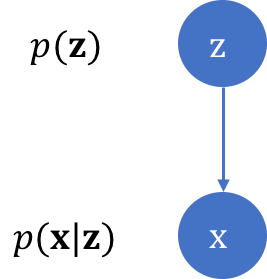
One can think of the mapping \(G\) as shaping the prior density to obtain a model density close to the data density. But when is such a density even well-defined on \(\mathbb{R}^d\) in the case of a GAN? One necessary requirement is that the dimensions of \(\mathbf{z}\) should be at least equal to the dimension of \(\mathbf{x}\) (e.g., if \(\mathbf{z}=\mathbb{R}\) and \(\mathbf{x}=\mathbb{R}^2\), then \(G(\mathbf{z})\) would trace a curve in this plane). Secondly, a density (=mass/volume) function in any space on \(\mathbb{R}^d\) is valid only if the probability mass is not concentrated in a region of non-zero volume in the transformed space and hence can integrate to 1 (with respect to the Lesbegue measure on \(\mathbb{R}^d\)). Intuitively, this implies that \(G\) should not transform every latent vector to a region of non-zero volume, such as the pathological case of a generator identically mapping every \(\mathbf{z}\) to the same \(\mathbf{x}\).³

The above discussion suggests that one sufficient requirement for obtaining well-defined likelihoods in a GAN is to learn an invertible (bijective) mapping between the latent space and the observed space. Invertibility would ensure that the dimensions of \(\mathbf{z}\) and \(\mathbf{x}\) are the same and avoid pathological cases such as the ones described above (where the measure defined by the model is not absolutely continuous with respect to the Lesbegue measure on \(\mathbb{R}^d\)), as long as the prior density is itself well-defined.

Normalizing flow models are one such class of models where an invertible generator \(G\) maps the latent variables \(\mathbf{z}\) to the observed variables \(\mathbf{x}\) such that \(\mathbf{x}=G(\mathbf{z})\) and \(G^{-1}\) exists. Geometrically, the transformation \(G\) causes an expansion (or contraction) of a volume defined in the two spaces. For illustrative purposes, consider a 1D setting with an invertible generator function \(G\). Since \(\mathbf{x}=G(\mathbf{z})\), we can differentiate both sides to get:

Hence the scaling factor for an infinitesmal volume around \(\mathbf{z}\) under the mapping \(G\) is given by the derivative of \(G\) evaluated at \(\mathbf{z}\). In particular, the volume expands if the quantity is greater than unity, contracts if the quantity is less than unity, and remains unchanged (a.k.a. volume preserving) if it equals unity.

We can now define likelihoods for the above generator. Let \(P(\cdot)\) denote the model distribution assumed to admit an absolutely continuous density denoted by lowercase \(p(\cdot)\), on a reference measure \(\mathrm{d}\mathbf{x}\). Noting that a continuous function in 1D is invertible iff the function is monotone, we can relate the distribution functions for an arbitrary point \(\mathbf{a} \in \mathbb{R}\) over the latent space and the observed space:

By differentiating the distribution functions on both sides with respect to \(\mathbf{x}\) and rearranging terms, we can obtain the corresponding densities for both the above cases:

The above derivation can also be extended to higher dimensions. In general, the likelihood of any \(d\)-dimensional point \(\mathbf{a} \in \mathbb{R}^d\) under a normalizing flow generator \(G\) is given by:

where \(\frac{\partial G^{-1}}{\partial \mathbf{x}}\) denotes the Jacobian of \(G^{-1}\) and the determinant is evaluated at \(\mathbf{x}=\mathbf{a}\). Hence we can efficiently evaluate exact likelihoods for a normalizing flow model as long as the prior density and determinant of the Jacobian above are tractable.⁴

In Flow-GANs, we propose to use the modeling assumptions corresponding to a normalizing flow model for specifying the generative process. An invertible Flow-GAN generator retains the assumptions of a deterministic observation model (as in a regular GAN but unlike a VAE), permits efficient ancestral sampling (as in any directed latent variable model), and allows for exact likelihood evaluation (unlike a VAE or a regular GAN)! Consequently, Flow-GANs can be learned using both maximum likelihood estimation and adversarial training.

Empirical evaluation

A Flow-GAN allows for a fair empirical comparison of the two learning paradigms: we are provided with the same reference data distribution and the same model family which implies that any differences in evaluation can arise only due to different learning objectives and optimization algorithms. With the rules of the game uniform, we can then ask the question:

Under a fixed set of modeling assumptions, how do the learning principles based on adversarial training (ADV) compare against maximum likelihood estimation (MLE) on held-out likelihoods and sampling metrics?

Subsequently, we perform experiments on the MNIST and CIFAR-10 datasets with NICE (Dinh, Krueger, and Bengio 2014) and Real-NVP (Dinh, Sohl-Dickstein, and Bengio 2017) generators respectively. We train both these generators based on MLE and ADV (in particular, the Wasserstein loss (Arjovsky, Chintala, and Bottou 2017)) objectives.

Our empirical analysis confirms some expected trends:

• MLE outperforms ADV on test log-likelihoods
• ADV outperforms MLE on sampling metrics

However, we find a suprising quantitative insight into the log-likelihoods attained by ADV. In particular, the log-likelihoods attained by ADV show a consistent decrease as training progresses and are orders of magnitude worse (100x and 10,000x worse for MNIST and CIFAR-10 respectively).

To put these results in perspective, we learn a simple Gaussian mixture model (GMM) baseline with a fixed bandwidth Gaussian centered at each of the training points. The plots below compares the held-out negative log-likelihoods (NLL) and sampling metrics (MODE/Inception scores) of the GMM for different bandwidths with those corresponding to the best ADV models.

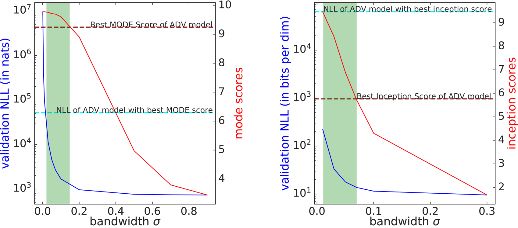
The green shaded region shows the range of bandwidths for which GMMs outperform ADV models on both held-out log-likelihoods and sampling metrics on MNIST (left) and CIFAR-10 (right).

The GMM can clearly attain better sampling metrics since it is explicitly overfitting to the training data, especially for low values of the bandwidth parameter (any \(\sigma\) for which the red curve is above the maroon dashed line). Surprisingly, the simple GMM also outperforms the adversarially learned model with respect to log-likelihoods attained for several values of the bandwidth parameter (any \(\sigma\) for which the blue curve is below the cyan dashed line).

A trivial baseline that is memorizing the training data can generate high quality samples and achieves better held-out log-likelihoods than adversarial learning!

Digging deeper to interpret the results

The above results present a somewhat concerning observation about adversarial learning and beg a more detailed understanding. Overfitting? Not quite since we find that the train and validation log-likelihood learning curves closely trace each other.

Mode collapse is the other commonly cited failure mode of ADV and qualitiatively indicates a lack of sample diversity but can be hard to detect and quantify. With a handle on the log-likelihoods however, we can formalize such a phenomena in Flow-GAN models. In particular, we inspect the conditoning of the Jacobian of the generator function \(G\) (evaluated at noise vectors randomly sampled from the prior) for models learned using MLE and ADV. Unlike the case of MLE, we find that the Jacobian for ADV are ill-conditioned that suggests the following result:

Adversarial learning shows a strong preference for distributions of low support.

To further the geometric intution, we find that models learned using ADV are trying to squish a sphere of unit volume centered at a point in the latent space to a very small volume in the observed space. Even tiny perturbations of data points hence manifest as poor log-likelihoods. Note that this is true in spite of the fact that an invertible generator is not limited in representational capacity to cover the entire space of the data distribution.

Combining maximum likelihood and adversarial learning

The dichotomy of good log-likelihoods attained using MLE and good sampling using ADV can be resolved to a large extent by combining these objectives to learn a Hybrid Flow-GAN with a hyperparameter controlling the relative importance. On CIFAR-10, the Hybrid model achieves the intended effect of balanced test log-likelihoods and Inception scores. To our surprise, we found such a combination to improve both log-likelihoods and MODE scores over MLE and ADV trained models for MNIST suggesting that ADV has a regularizing effect on MLE and MLE improves the mode coverage for ADV in this particular case. The Hybrid model corrects for the ill-conditioning of the Jacobian on both datasets.

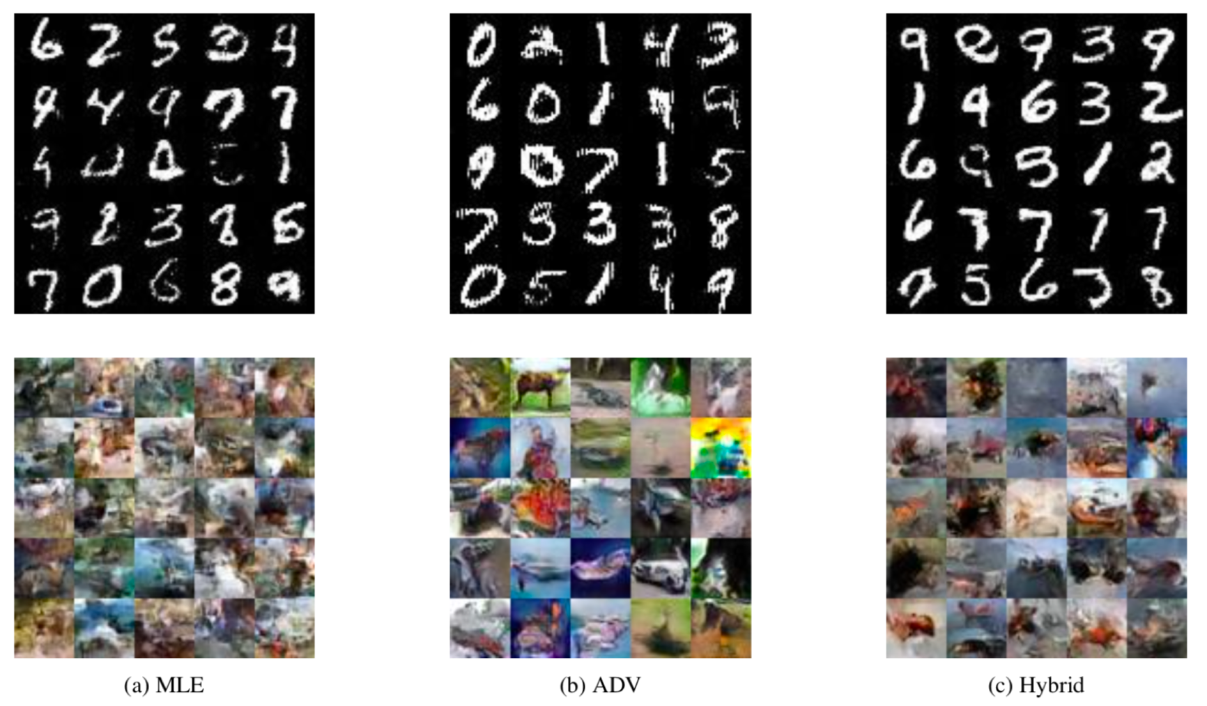
Samples generated by Flow-GAN models on MNIST (top) and CIFAR-10 (bottom).

Final thoughts

The merits of any generative model are closely linked with the learning procedure and the downstream inference task these models are applied to. Indeed, some tasks benefit immensely from models learning using maximum likelihood as opposed to adversarial learning (and vice versa). In Flow-GANs, we presented a framework for a principled quantitative comparison of these two learning paradigms under a uniform, restricted set of modeling assumptions corresponding to an invertible generator. We are optimistic that such a holistic perspective can guide future algorithmic as well as applied research in generative modeling. If you are interested in reading more about this research, check out the paper below:

Flow-GAN: Combining Maximum Likelihood and Adversarial Learning in Generative Models
Aditya Grover, Manik Dhar, and Stefano Ermon
AAAI Conference on Artificial Intelligence, 2018.
paper code

Footnotes

References

1. Mohamed, Shakir, and Balaji Lakshminarayanan. 2016. “Learning in Implicit Generative Models.” ArXiv Preprint ArXiv:1610.03483.
2. Hinton, Geoffrey E. 2002. “Training Products of Experts by Minimizing Contrastive Divergence.” Neural Computation 14 (8): 1771–1800.
3. Larochelle, Hugo, and Iain Murray. 2011. “The Neural Autoregressive Distribution Estimator.” In International Conference on Artificial Intelligence and Statistics, 29–37.
4. Kingma, Diederik P, and Max Welling. 2014. “Auto-Encoding Variational Bayes.” In International Conference on Learning Representations.
5. Dinh, Laurent, David Krueger, and Yoshua Bengio. 2014. “NICE: Non-Linear Independent Components Estimation.” ArXiv Preprint ArXiv:1410.8516.
6. Dinh, Laurent, Jascha Sohl-Dickstein, and Samy Bengio. 2017. “Density Estimation Using Real NVP.” In International Conference on Learning Representations.
7. Goodfellow, Ian, Jean Pouget-Abadie, Mehdi Mirza, Bing Xu, David Warde-Farley, Sherjil Ozair, Aaron Courville, and Yoshua Bengio. 2014. “Generative Adversarial Nets.” In Advances in Neural Information Processing Systems, 2672–80.
8. Salimans, Tim, Ian Goodfellow, Wojciech Zaremba, Vicki Cheung, Alec Radford, and Xi Chen. 2016. “Improved Techniques for Training Gans.” In Advances in Neural Information Processing Systems, 2226–34.
9. Che, Tong, Yanran Li, Athul Paul Jacob, Yoshua Bengio, and Wenjie Li. 2017. “Mode Regularized Generative Adversarial Networks.” In International Conference on Learning Representations.
10. Arjovsky, Martin, Soumith Chintala, and Léon Bottou. 2017. “Wasserstein GAN.” In International Conference on Machine Learning.
11. Nowozin, Sebastian, Botond Cseke, and Ryota Tomioka. 2016. “f-GAN: Training Generative Neural Samplers Using Variational Divergence Minimization.” In Advances in Neural Information Processing Systems.
12. Fedus, William, Mihaela Rosca, Balaji Lakshminarayanan, Andrew M Dai, Shakir Mohamed, and Ian Goodfellow. 2017. “Many Paths to Equilibrium: GANs Do Not Need to Decrease ADivergence At Every Step.” ArXiv Preprint ArXiv:1710.08446.
13. Wu, Yuhuai, Yuri Burda, Ruslan Salakhutdinov, and Roger Grosse. 2017. “On the Quantitative Analysis of Decoder-Based Generative Models.” In International Conference on Learning Representations.